10.6.3. LAMMPS Python Tutorial

Overview 

The lammps Python module is a wrapper class for the LAMMPS C language library interface API which is written using Python ctypes. The design choice of this wrapper class is to follow the C language API closely with only small changes related to Python specific requirements and to better accommodate object-oriented programming.

In addition to this flat ctypes interface, the lammps wrapper class exposes a discoverable API that doesn’t require as much knowledge of the underlying C language library interface or LAMMPS C++ code implementation.

Finally, the API exposes some additional features for IPython integration into Jupyter notebooks, e.g. for embedded visualization output from dump style image.

Quick Start 

Note

If you only want to use LAMMPS from Python and do not need to compile it yourself, you can also install a pre-compiled LAMMPS package that includes the Python module via conda.

System-wide or User Installation 

Step 1: Building LAMMPS as a shared library 

To use LAMMPS inside of Python it has to be compiled as shared library. This library is then loaded by the Python interface. In this example we enable the MOLECULE package and compile LAMMPS with PNG and JPEG output support enabled.

cd $LAMMPS_DIR

# MPI, PNG, JPEG, and FFMPEG support are auto-detected
cmake -S cmake -B build-shared -D PKG_MOLECULE=on -D PKG_PYTHON=on \
      -D PKG_GRAPHICS=on -D BUILD_SHARED_LIBS=on
cmake --build build-shared

cd $LAMMPS_DIR/src

# add LAMMPS packages if necessary
make yes-MOLECULE
make yes-PYTHON
make yes-GRAPHICS

# compile shared library using Makefile
make mpi mode=shlib LMP_INC="-DLAMMPS_PNG -DLAMMPS_JPEG" JPG_LIB="-lpng -ljpeg"

Step 2: Installing the LAMMPS Python module 

Next install the LAMMPS Python module into your current Python installation with:

cmake --build build-shared --target install-python

make install-python

This will create a so-called “wheel” and then install the LAMMPS Python module from that “wheel” either into a system folder (provided the command is executed with root privileges) or into your personal Python module folder.

Note

Recompiling the shared library requires re-installing the Python package.

Handling an “externally-managed-environment” Error

Some Python installations made through Linux distributions (e.g. Ubuntu 24.04LTS or later) will prevent installing the LAMMPS Python module into a system folder or a corresponding folder of the individual user as attempted by the install-python target with an error stating that an externally managed python installation must be only managed by the same package management tool. This is an optional setting, so not all Linux distributions follow it. The reasoning and explanations for this error can be found in the Python Packaging User Guide

These guidelines suggest to create a virtual environment and install the LAMMPS Python module there (see below). This is generally a good idea and the LAMMPS developers recommend this, too. If, however, you want to proceed and install the LAMMPS Python module regardless, you can install the “wheel” file (see above) manually with the pip command by adding the --break-system-packages flag.

Installation inside of a virtual environment 

You can use virtual environments to create a custom Python environment specifically tuned for your workflow.

Benefits of using a virtual environment 

isolation of your system Python installation from your development installation
installation can happen in your user directory without root access (useful for HPC clusters)
installing packages through pip allows you to get newer versions of packages than e.g., through the apt or dnf package managers (and without root access)
you can even install specific old versions of a package if necessary

Prerequisite (e.g. on Ubuntu)

sudo apt install python3-venv

Creating a virtual environment with LAMMPS installed 

# create virtual environment named 'testing'
python3 -m venv $HOME/python/testing

# activate 'testing' environment
source $HOME/python/testing/bin/activate

Now configure and compile the LAMMPS shared library as outlined above with the virtual environment active. CMake will then use the Python interpreter of the virtual environment. If the shared library has already been configured before the virtual environment was activated, you need to re-run CMake to update the location of the Python executable to the location in the virtual environment with:

cmake -S cmake -B build-shared -D Python_EXECUTABLE=$(which python)

Then install the LAMMPS Python module (for the traditional make build use make install-python in the src folder instead) and other useful packages into the virtual environment:

# install LAMMPS package in virtual environment
cmake --build build-shared --target install-python

# install other useful packages
pip install matplotlib jupyterlab mpi4py pandas

# ... use LAMMPS from Python ...

# return to the original shell environment
deactivate

Creating a new lammps instance 

To create a lammps object you need to first import the class from the lammps module. By using the default constructor, a new lammps instance is created.

from lammps import lammps
L = lammps()

See the LAMMPS Python documentation for how to customize the instance creation with optional arguments.

When the instance is no longer needed, it can be deleted with L.close(). Alternatively, the instance can be created in a with statement, and then it will be closed automatically at the end of the block:

with lammps() as L:
    L.command("units real")
    # ... more LAMMPS commands ...

Commands 

Sending a LAMMPS command with the library interface is done using the command method of the lammps object.

For instance, let’s take the following LAMMPS command:

region box block 0 10 0 5 -0.5 0.5

This command can be executed with the following Python code if L is a lammps instance:

L.command("region box block 0 10 0 5 -0.5 0.5")

For convenience, the lammps class also provides a command wrapper cmd that turns any LAMMPS command into a regular function call:

L.cmd.region("box block", 0, 10, 0, 5, -0.5, 0.5)

Note that each parameter is set as Python number literal. With the wrapper each command takes an arbitrary parameter list and transparently merges it to a single command string, separating individual parameters by white-space.

The benefit of this approach is avoiding redundant command calls and easier parameterization. With the command function each call needs to be assembled manually using formatted strings.

L.command(f"region box block {xlo} {xhi} {ylo} {yhi} {zlo} {zhi}")

The wrapper accepts parameters directly and will convert them automatically to a final command string.

L.cmd.region("box block", xlo, xhi, ylo, yhi, zlo, zhi)

Note

When running in IPython you can use Tab-completion after L.cmd. to see all available LAMMPS commands.

Accessing atom data 

All per-atom properties that are part of the atom style in the current simulation can be accessed using the extract_atom() method. This can be retrieved as ctypes objects or as NumPy arrays through the numpy property of the lammps object. Those represent the local atoms of the individual sub-domain for the current MPI process and may contain information for the local ghost atoms or not depending on the property. Both can be accessed as lists, but for the ctypes list object the size is not known and has to be retrieved first to avoid out-of-bounds accesses.

nlocal = L.extract_setting("nlocal")
nall = L.extract_setting("nall")
print("Number of local atoms ", nlocal, "  Number of local and ghost atoms ", nall)

# access via ctypes directly
atom_id = L.extract_atom("id")
print("Atom IDs", atom_id[0:nlocal])

# access through numpy wrapper
atom_type = L.numpy.extract_atom("type")
print("Atom types", atom_type)

x = L.numpy.extract_atom("x")
v = L.numpy.extract_atom("v")
print("positions array shape", x.shape)
print("velocity array shape", v.shape)
# turn on communicating velocities to ghost atoms
L.cmd.comm_modify("vel", "yes")
v = L.numpy.extract_atom('v')
print("velocity array shape", v.shape)

Some properties can also be set from Python since internally the data of the C++ code is accessed directly:

# set position in 2D simulation
x[0] = (1.0, 0.0)

# set position in 3D simulation
x[0] = (1.0, 0.0, 1.)

Retrieving the values of thermodynamic data and variables 

To access thermodynamic data from the last completed timestep, you can use the get_thermo() method, and to extract the value of (compatible) variables, you can use the extract_variable() method.

result = L.get_thermo("ke") # kinetic energy
result = L.get_thermo("pe") # potential energy

# value of an equal-style variable named "t"
result = L.extract_variable("t") / 2.0

Error handling 

LAMMPS uses C++ exceptions for errors, and the C language library interface captures and records them. The Python module checks for errors after each call into LAMMPS and then re-throws them as a Python exception. This way you can handle LAMMPS errors in the conventional way through the Python exception handling mechanism:

from lammps import lammps, MPIAbortException

L = lammps()
try:
    L.command("unknown_command")
except MPIAbortException as e:
    # error on only some of the MPI processes; LAMMPS cannot continue
    print("Fatal LAMMPS error:", e)
    raise
except Exception as e:
    # error on all MPI processes
    print("LAMMPS error:", e)

An MPIAbortException signals an error that happened on only some of the MPI processes, where LAMMPS would otherwise call MPI_Abort() to terminate all processes. Please see Handling LAMMPS errors for more details.

Warning

Capturing a LAMMPS exception in Python can still mean that the current LAMMPS process is in an illegal state and must be terminated. It is advised to save your data and terminate the Python instance as quickly as possible.

Using LAMMPS in IPython notebooks and Jupyter 

If the LAMMPS Python package is installed for the same Python interpreter as IPython, you can use LAMMPS directly inside of an IPython notebook inside of Jupyter. Jupyter is a powerful integrated development environment (IDE) for many dynamic languages like Python, Julia and others, which operates inside of any web browser. Besides auto-completion and syntax highlighting it allows you to create formatted documents using Markdown, mathematical formulas, graphics and animations intermixed with executable Python code. It is a great format for tutorials and showcasing your latest research.

To launch an instance of Jupyter simply run the following command inside your Python environment (this assumes you followed the Quick Start instructions):

jupyter lab

Interactive Python Examples 

Examples of IPython notebooks can be found in the python/examples/ipython subdirectory. To open these notebooks launch jupyter lab inside this directory and navigate to one of them. The README.md file in this directory describes how to set up a suitable virtual environment. If you compiled and installed a LAMMPS shared library with the GRAPHICS package with PNG and JPEG support and have FFmpeg installed, you should be able to rerun all of these notebooks. The notebooks run LAMMPS in serial, so the per-atom data of the local MPI process contains all atoms.

Validating a dihedral potential 

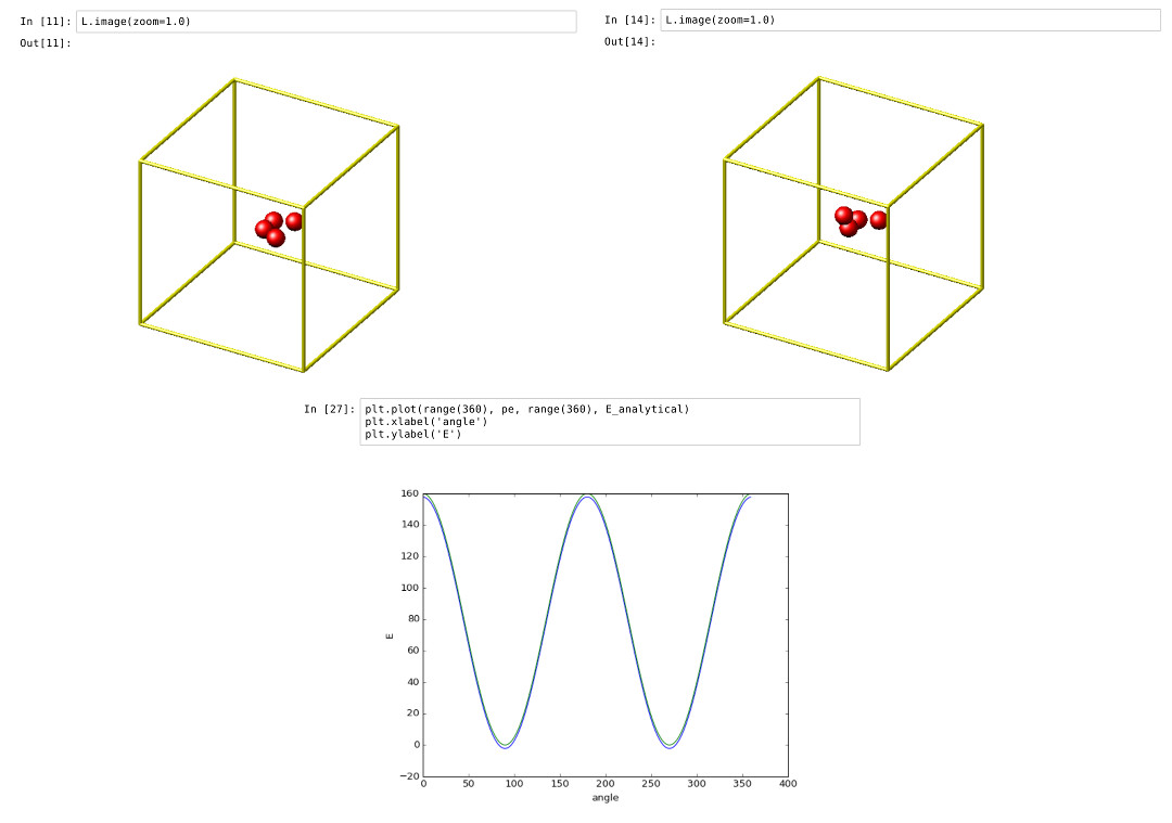
This example (dihedrals/dihedral.ipynb) showcases how an IPython Notebook can be used to compare a simple LAMMPS simulation of a harmonic dihedral potential to its analytical solution. Four atoms are placed in the simulation and the dihedral potential is applied on them using a datafile. Then one of the atoms is rotated along the central axis by setting its position from Python, which changes the dihedral angle.

phi = [d * math.pi / 180 for d in range(360)]

pos = [(1.0, math.cos(p), math.sin(p)) for p in phi]

x = L.numpy.extract_atom("x")

pe = []
for p in pos:
    x[3] = p
    L.cmd.run(0, "post", "no")
    pe.append(L.get_thermo("pe"))

By evaluating the potential energy for each position we can verify that trajectory with the analytical formula. To compare both solutions, we plot both trajectories over each other using matplotlib, which embeds the generated plot inside the IPython notebook.

Running a Monte Carlo relaxation 

This second example (montecarlo/mc.ipynb) shows how to use the lammps Python interface to create a 2D Monte Carlo Relaxation simulation, computing and plotting energy terms and even embedding video output.

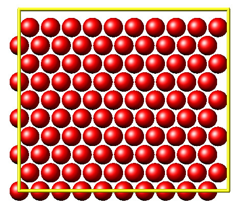
Initially, a 2D system is created in a state with minimal energy.

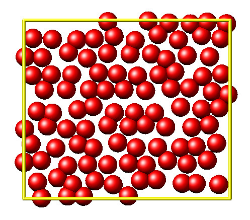
It is then disordered by moving each atom by a random delta.

random.seed(27848)
deltaperturb = 0.2

pos = L.numpy.extract_atom("x")
for i in range(len(pos)):
    x, y = pos[i][0], pos[i][1]
    dx = deltaperturb * random.uniform(-1, 1)
    dy = deltaperturb * random.uniform(-1, 1)
    pos[i] = (x+dx, y+dy, 0)

L.cmd.run(0, "post", "no")

Finally, the Monte Carlo algorithm is implemented in Python. It continuously moves random atoms by a random delta and only accepts certain moves.

estart = L.get_thermo("pe")
elast = estart

naccept = 0
energies = [estart]

niterations = 3000
deltamove = 0.1
kT = 0.05

natoms = L.extract_global("natoms")

for i in range(niterations):
    pos = L.numpy.extract_atom("x")
    iatom = random.randrange(0, natoms)
    current_atom = pos[iatom]

    x0, y0 = current_atom[0], current_atom[1]

    dx = deltamove * random.uniform(-1, 1)
    dy = deltamove * random.uniform(-1, 1)

    pos[iatom] = (x0+dx, y0+dy, 0)

    L.cmd.run(1, "pre no post no")

    e = L.get_thermo("pe")
    energies.append(e)

    if e <= elast:
        naccept += 1
        elast = e
    elif random.random() <= math.exp(natoms*(elast-e)/kT):
        naccept += 1
        elast = e
    else:
        pos[iatom] = (x0, y0, 0)

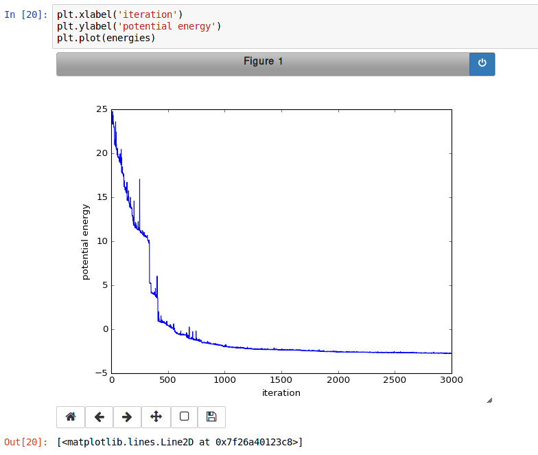
The energies of each iteration are collected in a Python list and finally plotted using matplotlib.

The IPython notebook also shows how to use dump commands and embed video files inside of the IPython notebook.