10.5.13. Smoothed particle hydrodynamics (SPH)

written by Georg C. Ganzenmueller, Martin O. Steinhauser, and Paul Van Liedekerke in 2011; converted from SPH_LAMMPS_userguide.pdf to reStructuredText and updated for current LAMMPS by Axel Kohlmeyer in 2026

The SPH package implements the smoothed particle hydrodynamics (SPH) method for fluids. This Howto gives a concise introduction to SPH, explains how the method is implemented in LAMMPS, and discusses the example inputs in the examples/PACKAGES/sph folder.

Overview 

SPH is a continuum method that does not require a predefined grid to evaluate the partial differential equations of continuum mechanics. Instead, SPH discretizes the mass distribution of a material into point masses (particles) which move with the material according to Newton’s equations of motion. The positions of these particles serve as integration points for the field equations. The required fields, for example the mass density or the pressure, are constructed on the fly by interpolation with kernel functions, which are centered at the particles. Due to this particle nature, SPH fits well into the data structures and the parallelization of LAMMPS: the SPH interactions are implemented as pair styles and the time integration as fixes.

The SPH package provides:

the atom style sph, which adds the local density, internal energy, heat capacity, and an extrapolated velocity to each particle,
pair styles for several equations of state with artificial or laminar viscosity (sph/taitwater, sph/taitwater/morris, sph/idealgas, sph/lj), for heat conduction (sph/heatconduction), and for computing the density by kernel summation (sph/rhosum),
the time integration fixes fix sph and fix sph/stationary,
the computes sph/rho/atom, sph/e/atom, and sph/t/atom for output of the per-particle SPH quantities,
keywords sph/rho, sph/e, and sph/cv for the set command to initialize these quantities.

Related methods are available in other packages: the MACHDYN package applies SPH to solids and fluids with material strength, see the Howto machdyn page, and the RHEO package offers a different SPH implementation for fluids and solids with additional features such as thermal coupling, phase transitions, and surface tension, see the Howto rheo page.

Quick start 

The SPH package is an optional package. If your LAMMPS executable does not already include it, see the Build package page for how to enable it when compiling LAMMPS from source.

The following input is a two-dimensional version of the shock tube problem discussed below. It contains all elements needed for an SPH simulation of a compressible fluid:

dimension     2
atom_style    sph
boundary      s p p

region        box block -100 150 -4 4 -0.1 0.1 units box
create_box    2 box
lattice       sq 1.0
create_atoms  1 box
region        right block 1 EDGE EDGE EDGE EDGE EDGE units box
set           region right type 2

mass          1 1.0
mass          2 0.25
set           type 1 sph/rho 1.0
set           type 2 sph/rho 0.25
set           type 1 sph/e 2.5
set           type 2 sph/e 0.625

pair_style    hybrid/overlay sph/rhosum 1 sph/idealgas
pair_coeff    * * sph/rhosum 4.0
pair_coeff    * * sph/idealgas 0.75 4.0

compute       rho all sph/rho/atom
compute       ie all sph/e/atom
compute       esph all reduce sum c_ie
variable      etot equal ke+c_esph
thermo_style  custom step ke c_esph v_etot
thermo_modify norm no
thermo        50

fix           1 all sph
fix           2 all setforce NULL 0.0 0.0
timestep      0.05
run           400

Some notes on this input:

The atom style sph is required. The particle mass is set per atom type with the mass command.
Each SPH particle needs an initial local density and internal energy, here set with the set command. The internal energy E stored by LAMMPS is the energy per particle and not the energy per unit mass e, i.e. \(E = m e\). For the ideal gas equation of state \(p = (\gamma - 1)\rho e\) with \(\gamma = 1.4\), the chosen values correspond to a pressure of 1.0 for type 1 and 0.25 for type 2.
The pair style sph/idealgas computes the pressure forces and artificial viscosity (with \(\alpha = 0.75\)), and the rates of change of the local density and internal energy. The pair style sph/rhosum recomputes the local density by kernel summation, here every step. Both use a kernel function with a range h of 4 lattice spacings, which is also the cutoff of the pair style.
Fix sph integrates the positions, velocities, local densities, and internal energies in time. The fix setforce command zeroes the forces in y and z direction to turn this into a quasi one-dimensional problem.
The total energy of the fluid is the sum of the kinetic energy and the internal energy of all particles. It is monitored with the help of the sph/e/atom and reduce computes.

SPH theory 

This section gives a concise introduction to SPH for fluids. For more detailed information, please see the books by Hoover (Hoover2006) and by Liu and Liu (Liu and Liu); this Howto follows the presentation in the book by Hoover. SPH solves the equations of continuum mechanics in the Lagrangian frame, where the governing partial differential equations describe the co-moving evolution of the mass density \(\rho\), the velocity \(\mathbf{v}\), and the internal energy per unit mass \(e\) in terms of gradients of the velocity, the pressure tensor \(\mathbf{P}\), and the heat flux \(\mathbf{Q} = -\kappa\nabla T\) with thermal conductivity \(\kappa\) and temperature \(T\):

\[\begin{split}\frac{d\rho}{dt} & = -\rho\,\nabla\cdot\mathbf{v} \\ \frac{d\mathbf{v}}{dt} & = -\frac{1}{\rho}\,\nabla\cdot\mathbf{P} \\ \frac{de}{dt} & = -\frac{1}{\rho}\,\mathbf{P} : \nabla\mathbf{v} - \frac{1}{\rho}\,\nabla\cdot\mathbf{Q}\end{split}\]

where \(\mathbf{A}:\mathbf{B} = \sum_{\alpha\beta} A_{\alpha\beta}B_{\alpha\beta}\) denotes the double contraction of two tensors.

Kernel interpolation 

SPH interpolates any field \(f(\mathbf{r})\) at the position \(\mathbf{r}_i\) of particle i as a weighted sum over the values \(f_j\) carried by its neighbor particles j:

\[f(\mathbf{r}_i) = \sum_j \frac{m_j}{\rho_j}\, f_j\, W(r_{ij}, h)\]

Here \(m_j\) and \(\rho_j\) are the mass and the local density of particle j, \(\mathbf{r}_{ij} = \mathbf{r}_i - \mathbf{r}_j\), and \(r_{ij} = |\mathbf{r}_{ij}|\). The kernel (or weight) function \(W\) is radially symmetric, normalized to unity, and has compact support: it decays to zero at the distance h, which in LAMMPS is the cutoff of the pair style and typically spans a few inter-particle spacings. Thus, only the particles within the distance h contribute to the sum. The interpolation turns the coupled set of partial differential equations above into a set of ordinary differential equations for the particles.

Since \(m_j\) and \(f_j\) are particle properties, the gradient operator only acts on the kernel function:

\[\nabla f(\mathbf{r}_i) = \sum_j \frac{m_j}{\rho_j}\, f_j\, \nabla_i W_{ij}, \qquad \nabla_i W_{ij} = \frac{\mathbf{r}_{ij}}{r_{ij}}\, \frac{\partial W(r_{ij})}{\partial r_{ij}}\]

Because of the radial symmetry of \(W\), the kernel gradient is antisymmetric: \(\nabla_i W_{ij} = -\nabla_j W_{ij}\).

Local density 

Setting \(f \equiv \rho\) in the interpolation gives the SPH expression for the local density, which includes the contribution of particle i itself:

\[\rho_i = \sum_j m_j W_{ij}\]

The local density computed this way is a smoothed quantity with contributions from all particles within the distance h.

Equation of motion 

To obtain a computable expression for the acceleration, the divergence of the pressure tensor is rewritten with the identity

\[-\frac{1}{\rho}\,\nabla\cdot\mathbf{P} \equiv -\nabla\cdot\frac{\mathbf{P}}{\rho} - \frac{\mathbf{P}}{\rho^2}\cdot\nabla\rho\]

and both gradients on the right-hand side are discretized with the SPH gradient expression. For a fluid with a scalar pressure \(P\), this leads to a sum of pairwise forces:

\[\mathbf{f}_i = m_i \frac{d\mathbf{v}_i}{dt} = -\sum_j m_i m_j \left( \frac{P_i}{\rho_i^2} + \frac{P_j}{\rho_j^2} \right) \nabla_i W_{ij}\]

Due to the antisymmetry of the kernel gradient, the pair forces obey Newton’s third law and the SPH discretization conserves the total linear momentum.

Continuity equation 

Rewriting the continuity equation with the identity \(\nabla\cdot(\rho\mathbf{v}) = \rho\nabla\cdot\mathbf{v} + \mathbf{v}\cdot\nabla\rho\) and applying the SPH gradient expression gives the rate of change of the local density in terms of the relative velocities \(\mathbf{v}_{ij} = \mathbf{v}_i - \mathbf{v}_j\):

\[\frac{d\rho_i}{dt} = \sum_j m_j\, \mathbf{v}_{ij}\cdot\nabla_i W_{ij}\]

Energy equation 

Proceeding in the same way for the energy equation, the rate of change of the internal energy \(E_i = m_i e_i\) of particle i due to compression or expansion is:

\[\frac{dE_i}{dt} = \frac{1}{2} \sum_j m_i m_j \left( \frac{P_i}{\rho_i^2} + \frac{P_j}{\rho_j^2} \right) \mathbf{v}_{ij}\cdot\nabla_i W_{ij}\]

The energy change due to heat conduction is discussed below.

Artificial viscosity 

Numerical integration of the compressible Navier-Stokes equations is generally unstable in the sense that small pressure waves can steepen due to numerical artifacts and turn into shock waves. To suppress this source of instability, Monaghan introduced an extension of the von Neumann-Richtmyer artificial viscosity into SPH (Monaghan). An additional viscous term \(\Pi_{ij}\) is added to the pressure terms in the force and energy expressions:

\[\begin{split}\mathbf{f}_i & = -\sum_j m_i m_j \left( \frac{P_i}{\rho_i^2} + \frac{P_j}{\rho_j^2} + \Pi_{ij} \right) \nabla_i W_{ij} \\ \frac{dE_i}{dt} & = \frac{1}{2}\sum_j m_i m_j \left( \frac{P_i}{\rho_i^2} + \frac{P_j}{\rho_j^2} + \Pi_{ij} \right) \mathbf{v}_{ij}\cdot\nabla_i W_{ij}\end{split}\]

with

\[\Pi_{ij} = -\alpha\, \frac{c_i + c_j}{\rho_i + \rho_j}\; \frac{h\, \mathbf{v}_{ij}\cdot\mathbf{r}_{ij}}{r_{ij}^2 + \epsilon h^2} \quad\text{for}\quad \mathbf{v}_{ij}\cdot\mathbf{r}_{ij} < 0, \qquad \Pi_{ij} = 0 \quad\text{otherwise}\]

Here, \(c_i\) and \(c_j\) are the speeds of sound of particles i and j, \(\alpha\) is a dimensionless factor controlling the strength of the dissipation, and \(\epsilon = 0.01\) avoids a singularity when particles are very close. The viscous term only acts between particles that approach each other. Following (Gonzalez), the artificial viscosity can be related to an effective kinematic viscosity \(\nu \approx \alpha h c / 8\).

Laminar flow viscosity 

While the artificial viscosity usually gives good results for turbulent flows, the velocity profiles of flows at low Reynolds numbers may be inaccurate. Morris et al. (Morris) proposed an expression for the viscous term of the Navier-Stokes equations similar to the one used for heat conduction. With a dynamic viscosity \(\mu = \rho\nu\), the viscous force and the corresponding viscous heating are:

\[\begin{split}\mathbf{f}_i^\text{visc} & = \sum_j \frac{2 m_i m_j \mu}{\rho_i \rho_j}\, \frac{1}{r_{ij}}\frac{\partial W}{\partial r_{ij}}\; \mathbf{v}_{ij} \\ \left.\frac{dE_i}{dt}\right|^\text{visc} & = -\frac{1}{2}\sum_j \frac{2 m_i m_j \mu}{\rho_i \rho_j}\, \frac{1}{r_{ij}}\frac{\partial W}{\partial r_{ij}}\; v_{ij}^2\end{split}\]

These terms replace the artificial viscosity in the force and energy expressions.

Time step 

As for any explicit time integration scheme, the time step \(\Delta t\) must be small enough that information cannot propagate farther than a fraction of the kernel range per step. This Courant-Friedrichs-Lewy (CFL) criterion is typically formulated as \(\Delta t \le C_\text{CFL}\, h / c\), with c the speed of sound and \(C_\text{CFL}\) about 0.1 to 0.3. For laminar flows, the time step can be limited by viscous diffusion rather than by the CFL criterion. A stable simulation should then also fulfill \(\Delta t < 0.125\, h^2/\nu\).

Implementation in LAMMPS 

Per-particle data 

LAMMPS provides data structures for positions, velocities, and forces. SPH requires at least four additional per-particle quantities: the local density \(\rho\), the internal energy \(E = m e\), and their time derivatives \(\dot\rho\) and \(\dot E\). These are added by the atom style sph, which also stores a per-particle heat capacity \(C_V\), so that a per-particle temperature \(T = E/C_V\) can be computed, and an extrapolated velocity (see below). With both \(\rho\) and \(E\) available, complete equations of state, i.e. equations of state that depend on density and temperature, are supported.

Kernel functions 

All SPH pair styles have the kernel range h as their last pair_coeff parameter, which is also the cutoff of the interaction. The pair styles that compute forces, heat conduction, and density changes use the Lucy kernel (Lucy), while the pair style sph/rhosum uses a quartic polynomial kernel, which does not require evaluating a square root:

\[\begin{split}W_\text{Lucy}(r < h) & = \frac{1}{s} \left( 1 + 3\frac{r}{h} \right) \left( 1 - \frac{r}{h} \right)^3 \\ W_\text{quartic}(r < h) & = \frac{1}{s} \left( 1 - \frac{r^2}{h^2} \right)^4\end{split}\]

The normalization constants s depend on the dimension of the system; both two- and three-dimensional systems are supported.

Time integration 

LAMMPS integrates the equations of motion with the velocity-Verlet algorithm. This scheme cannot be used unchanged for SPH, because the velocities lag behind the positions by half a time step when the forces are computed. Since the SPH expressions for the density and energy changes depend explicitly on the velocities, this would lead to poor conservation of mass and energy. The situation is improved by computing an extrapolated velocity

\[\tilde{\mathbf{v}}_i(t + \Delta t) = \mathbf{v}_i(t) + \frac{\Delta t}{m_i}\,\mathbf{f}_i(t)\]

before the forces are computed, and using \(\tilde{\mathbf{v}}\) in all SPH pair styles. This extrapolation is only accurate to first order in \(\Delta t\). The local density and the internal energy are integrated in two half steps, in analogy to the velocities, since a simple Euler integration of these quantities would lead to poor energy conservation. The complete scheme implemented by fix sph for each time step reads:

\(\mathbf{v}_i(t + \frac{1}{2}\Delta t) = \mathbf{v}_i(t) + \frac{\Delta t}{2 m_i}\mathbf{f}_i(t)\)
\(\tilde{\mathbf{v}}_i(t + \Delta t) = \mathbf{v}_i(t) + \frac{\Delta t}{m_i}\mathbf{f}_i(t)\)
\(\rho_i(t + \frac{1}{2}\Delta t) = \rho_i(t) + \frac{\Delta t}{2}\dot\rho_i(t)\) and \(E_i(t + \frac{1}{2}\Delta t) = E_i(t) + \frac{\Delta t}{2}\dot E_i(t)\)
\(\mathbf{r}_i(t + \Delta t) = \mathbf{r}_i(t) + \Delta t\,\mathbf{v}_i(t + \frac{1}{2}\Delta t)\)
compute \(\mathbf{f}_i(t + \Delta t)\), \(\dot\rho_i(t + \Delta t)\), and \(\dot E_i(t + \Delta t)\) with the pair styles
\(\rho_i(t + \Delta t) = \rho_i(t + \frac{1}{2}\Delta t) + \frac{\Delta t}{2}\dot\rho_i(t + \Delta t)\) and \(E_i(t + \Delta t) = E_i(t + \frac{1}{2}\Delta t) + \frac{\Delta t}{2}\dot E_i(t + \Delta t)\)
\(\mathbf{v}_i(t + \Delta t) = \mathbf{v}_i(t + \frac{1}{2}\Delta t) + \frac{\Delta t}{2 m_i}\mathbf{f}_i(t + \Delta t)\)

Fix sph/stationary integrates only the local density and the internal energy and leaves positions and velocities unchanged. It is used for boundary particles, see below.

Since the SPH equations are stiff, the time step is often chosen adaptively with the fix dt/reset command, which reduces the time step during violent parts of a flow and enlarges it when the flow calms down. This is demonstrated in the water collapse example below.

Local density 

The pair styles that compute forces also compute the rate of change of the local density from the continuity equation, which is then integrated in time by the fix. This requires a consistent initial value for the local density of each particle, which can be set with the sph/rho keyword of the set command or read from a data file. The initial densities must be consistent with the particle masses and the particle spacing, otherwise the results will be poor.

Alternatively, the local density can be recomputed from scratch with the kernel summation by adding the pair style sph/rhosum through pair_style hybrid/overlay. Its argument Nstep determines how often the summation is performed. On all other steps, the density is updated with the continuity equation. The summation underestimates the density of particles close to a free surface or a boundary, where neighbors are missing. In the water collapse example below, the summation is therefore only applied to the water particles but not to the boundary particles.

Equations of state 

The equation of state determines the pressure as a function of the local density and, for complete equations of state, the internal energy. Each equation of state is implemented as a separate pair style that also includes the viscosity model:

Pair style	Equation of state	Viscosity
sph/taitwater	Tait equation of state for water	artificial viscosity
sph/taitwater/morris	Tait equation of state for water	laminar viscosity (Morris)
sph/idealgas	ideal gas with \(\gamma = 1.4\)	artificial viscosity
sph/lj	Lennard-Jones fluid	artificial viscosity

The Tait equation of state

\[P(\rho) = \frac{c_0^2\rho_0}{7}\left[ \left( \frac{\rho}{\rho_0} \right)^7 - 1 \right]\]

is an incomplete equation of state devised to model water at ambient conditions; \(c_0\) and \(\rho_0\) are the speed of sound and the density at zero pressure. For simulations of incompressible flows, it is common to choose a speed of sound much smaller than that of real water, but still about ten times larger than the largest flow velocity, so that density fluctuations remain small while the time step can be much larger. The ideal gas equation of state \(P = (\gamma - 1)\rho e\) uses a fixed heat capacity ratio \(\gamma = C_p/C_V = 1.4\), corresponding to dry air. The Lennard-Jones equation of state is the continuum equivalent of a fluid of particles interacting with the Lennard-Jones pair potential. It uses the parametrization of Ree (Ree) with \(\epsilon\) and \(\sigma\) set to unity.

Heat conduction 

Heat conduction between SPH particles is computed by the pair style sph/heatconduction. It only changes the internal energy of the particles,

\[\left.\frac{dE_i}{dt}\right|^\text{cond} = \sum_j \frac{2 m_i m_j}{m_i + m_j}\, \frac{\rho_i + \rho_j}{\rho_i \rho_j}\, D\, (E_i - E_j)\, \frac{1}{r_{ij}}\frac{\partial W}{\partial r_{ij}}\]

where D is the heat diffusion coefficient (thermal diffusivity) with units of length²/time. It is related to the thermal conductivity by \(D = \kappa/(\rho c_V)\), with \(c_V\) the heat capacity per unit mass. To combine heat conduction with fluid flow, the pair style is added through pair_style hybrid/overlay.

Boundary conditions 

In macroscopic simulations, it is often desirable to confine a fluid to a region of space. One possibility is to use one of the fix wall commands. However, such walls result in poor energy conservation. It is usually better to represent the walls with stationary SPH particles, which take part in the SPH summations, but are only integrated with fix sph/stationary, so that only their local density and internal energy change. Please note that even though these boundary particles have zero velocity, the SPH interpolated velocity at their positions is not zero. This results in errors near the boundary, e.g. for the velocity profile of a laminar flow.

Initialization and output 

The local density, internal energy, and heat capacity of the particles can be set with the sph/rho, sph/e, and sph/cv keywords of the set command or read from the Atoms section of a data file. The format of a line in that section for atom style sph is given on the read_data page.

The current values of these quantities can be output with the computes sph/rho/atom, sph/e/atom, and sph/t/atom (temperature \(T = E/C_V\)), or with the rho, drho, e, de, and cv properties of compute property/atom. The resulting per-atom vectors can be used with dump custom, or summed up for thermodynamic output with compute reduce. For a quick look at a simulation, the dump image command can color the particles by any of these quantities.

Examples 

The following examples are included in the examples/PACKAGES/sph folder. They also served as validation tests of the implementation. Some of the inputs run only a small number of time steps by default, so that they can be used for regression testing. The number of steps is then set by the index style variable nsteps, which can be changed with the -var command-line switch, e.g. lmp -in in.water_collapse -var nsteps 50000. The README file in the folder lists the values needed for the complete examples, which were used for the figures below.

Heat conduction 

The input heatconduction/in.sph_heat_conduction_2d sets up a 2d bar of SPH particles with dimensions 100 cm by 10 cm and a particle spacing of 1 cm in SI units. The left half is assigned an internal energy of 1 J per particle, the right half 2 J per particle. Heat flows from right to left with a heat diffusion coefficient of \(1.0 \times 10^{-4}\) m²/s. All particles are integrated with fix sph/stationary, so they do not move, and there is neither potential nor kinetic energy. The total energy is thus the sum of the internal energies, which is computed and output with:

set             group all sph/rho 0.1 # = particle mass / particle area
pair_style      sph/heatconduction
#               i j diffusion coeff. cutoff
pair_coeff      1 1 1.0e-4           2.0e-2

compute         ie_atom all sph/e/atom
compute         ie all reduce sum c_ie_atom
thermo_style    custom step temp c_ie
fix             integrate_fix all sph/stationary

The analytic solution to this problem is obtained from the 1d diffusion equation:

\[E(x,t) = E_l + \frac{E_r - E_l}{2}\left[ 1 + \text{erf} \left( \frac{x - x_c}{\sqrt{4 D t}} \right) \right]\]

Here, \(E_l\) and \(E_r\) are the initial energies on the left and right sides, \(x_c\) is the position of the contact between the cold and hot regions, D is the diffusion coefficient, and t is time. The figure below shows the good agreement between the SPH results and the analytic solution. The folder also contains a 3d version of this example and a gnuplot script that compares the final profile with the analytic solution.

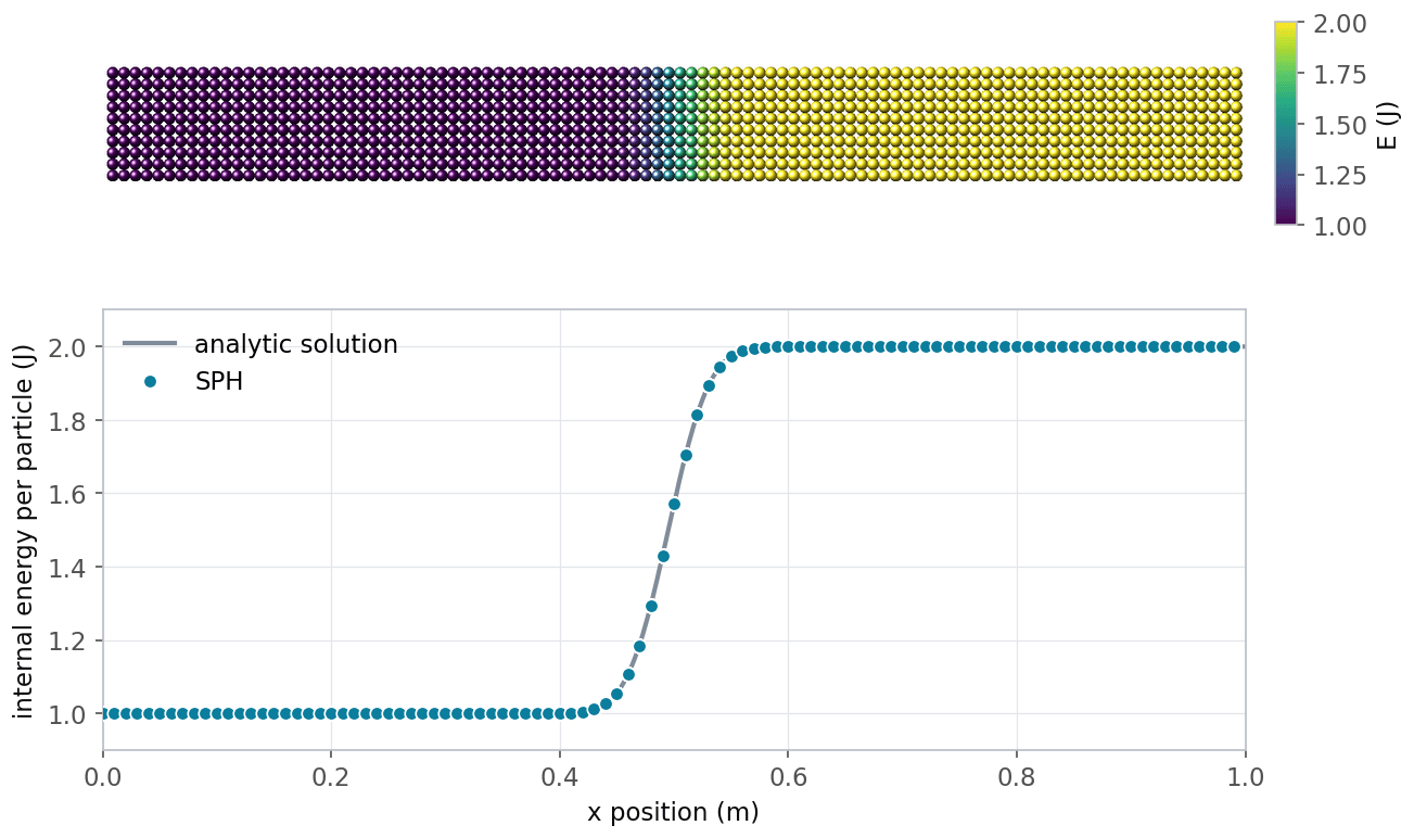
_images/sph-heat-conduction.png — Heat conduction example at t = 4 s. Top: the particles colored by their internal energy. Bottom: internal energy of the particles as a function of their position compared to the analytic solution.

Shock tube 

This example considers the solution of a quasi-1d shock wave problem in 2 or 3 dimensions (inputs shock_tube/in.shock2d and shock_tube/in.shock3d). It is adapted from Monaghan’s investigation of the performance of SPH for a 1d shock wave problem (Monaghan). In reduced units, the initial conditions are two regions of an ideal gas: a high density region on the left with \(P = \rho = 1\) in contact with a low density region on the right with \(P = \rho = 0.25\). As the high density gas expands into the low density region, a shock wave travels to the right while a rarefaction wave travels to the left. The particles are arranged on a square (simple cubic) lattice with spacing 1, extending from x = -100 to 150 and y = -4 to 4 (and z = -4 to 4 in 3d), with periodic boundaries in y and z. The particles with negative x coordinate have mass 1 and those with positive x coordinate have mass 0.25. The density is computed by kernel summation every step, and the artificial viscosity parameter is \(\alpha = 0.75\). The 2d input is very similar to the quick start example above.

The SPH results agree well with the exact solution of the corresponding Riemann problem, which is included in the file shock_tube/exact_solution.dat. The shock front and the contact discontinuity are smeared out over a distance of about h. The total energy, i.e. the sum of kinetic and internal energy, is conserved to better than one part per million.

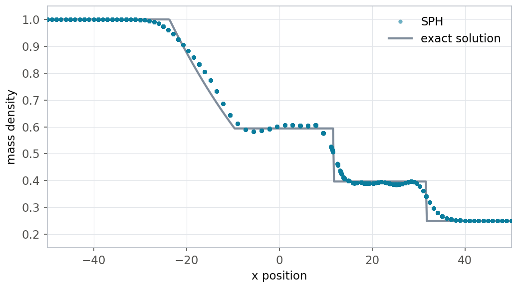
_images/sph-shock-tube.png — Mass density of the particles in the 3d shock tube example at t = 20 (400 steps) compared to the exact solution.

Collapse of a water column 

The input water_collapse/in.water_collapse simulates a prototypical test for SPH: the collapse of a water column in a rectangular container with an obstacle (Gomez-Gesteira). The geometry is read from the data file data.initial: a water column of 1 m by 2 m (type 1) in a container with a wedge-shaped obstacle that is represented by stationary SPH particles (type 2). Water is modeled with the Tait equation of state with \(c_0 = 10\) m/s, \(\rho_0 = 1000\) kg/m³, and an artificial viscosity of \(\alpha = 1\). The density of the water particles is recomputed by kernel summation every step.

variable     h equal 0.03
variable     c equal 10.0 # soundspeed for Tait's EOS
variable     dt equal 0.1*${h}/${c} # upper limit of timestep from CFL criterion

pair_style   hybrid/overlay sph/rhosum 1 sph/taitwater
pair_coeff   * * sph/taitwater 1000.0 ${c} 1.0 ${h}
pair_coeff   1 1 sph/rhosum ${h}

fix          gfix water gravity -9.81 vector 0 1 0
fix          2d_fix all enforce2d
# variable timestep: the fastest particle moves at most 0.0005 m per step
fix          dtfix all dt/reset 1 NULL ${dt} 0.0005 units box
fix          integrate_water_fix water sph
fix          integrate_bc_fix bc sph/stationary

The fix gravity command applies a downward force and also computes the potential energy of the water in the gravitational field, which is needed to monitor the conservation of the total energy. To deal efficiently with the time integration, a variable time step is used: the time step is chosen such that the fastest particle may move no more than 0.0005 m per step. Additionally, the time step is limited by the CFL criterion \(\Delta t < 0.1 h/c\).

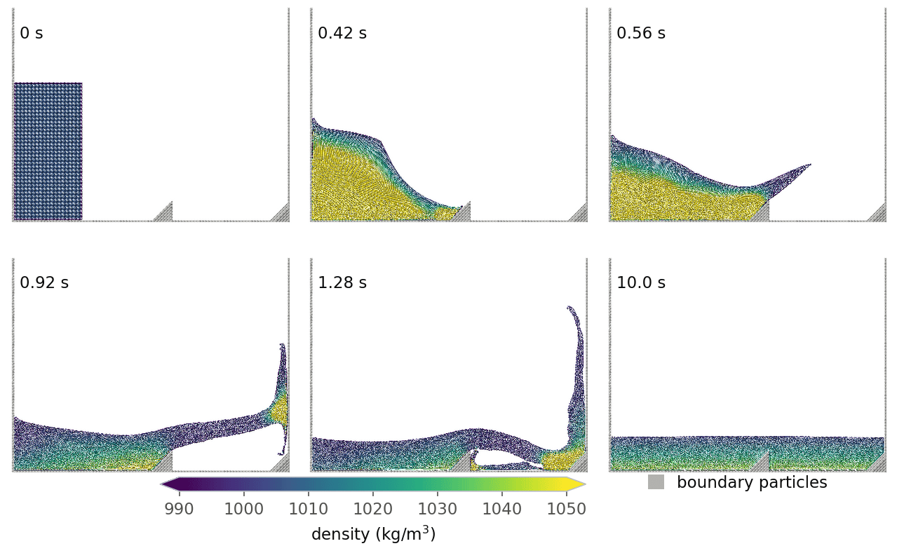
_images/sph-water-collapse.png — Snapshots of the water collapse example (lower part of the container). The water particles are colored by their local density and the boundary particles are gray. As the water column collapses, a wave splashes over the obstacle and hits the right container wall before the water settles.

The importance of the variable time step is demonstrated in the next figure. If a fixed time step were used instead, it would need to be set to the smallest value attained in this simulation to achieve the same degree of energy conservation. In contrast, the variable time step is only reduced when needed during the violent initial collapse of the column, when kinetic energy is converted into internal energy by viscous dissipation, and not during the comparatively well-ordered flow afterwards. The total energy is conserved to about 25 parts per million.

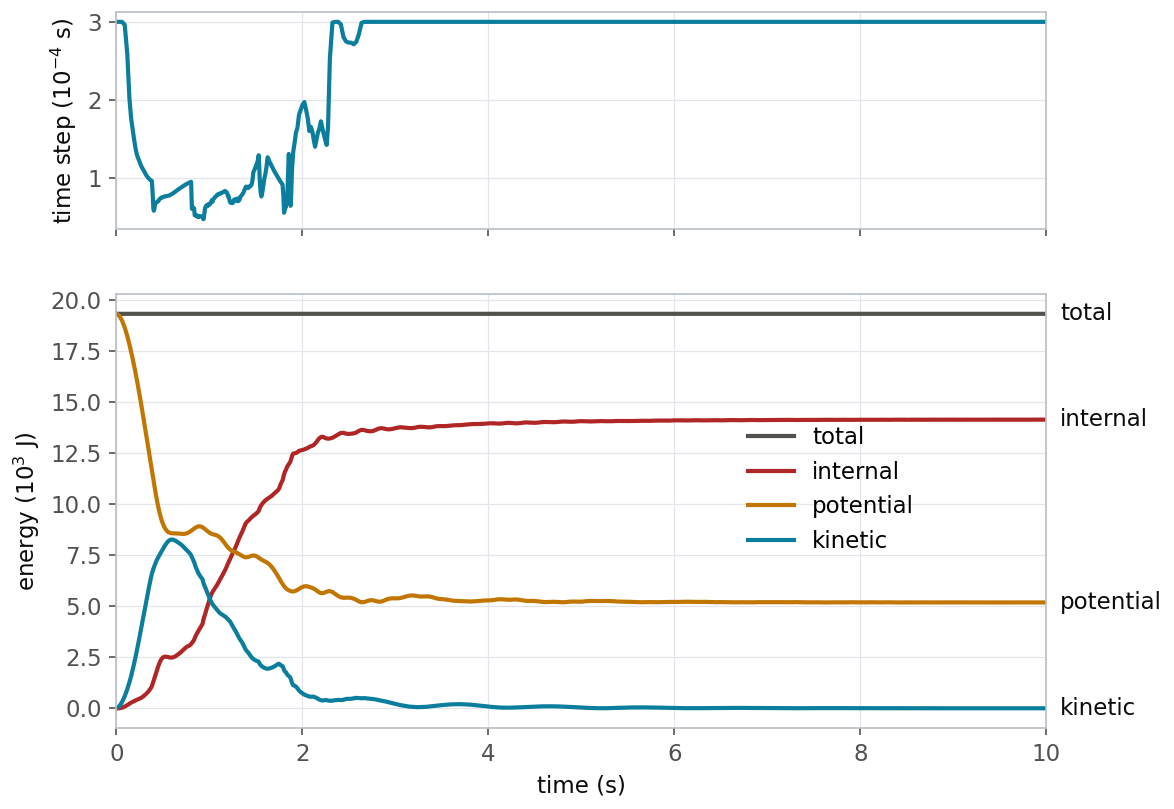
_images/sph-water-collapse-energy.png — Water collapse example. Top: time step selected by fix dt/reset. Bottom: kinetic energy, internal energy, potential energy in the gravitational field, and total energy.

Shear cavity flow 

The shear-driven cavity flow is a standard test for laminar flow (input cavity_flow/in.cavity_flow). A 2d square of fluid particles is enclosed by stationary wall particles on three sides (type 2), while a strip of particles on top (type 3) moves at a constant speed of \(10^{-3}\) m/s. The fluid is modeled with the Tait equation of state combined with the laminar flow viscosity of Morris et al., with a kinematic viscosity of \(\nu = 10^{-6}\) m²/s. The moving strip is integrated with fix sph, while its forces are set to zero with fix setforce, so that it keeps its velocity. Interactions between the walls and the moving strip are turned off.

pair_style   hybrid sph/taitwater/morris
#            rho0 c0  viscosity h
pair_coeff   * * sph/taitwater/morris 1000 0.1 1.0e-3 6.5e-5
pair_coeff   2 3 none # exclude interaction between walls and shear driver

velocity     driver set 0.001 0.0 0.0 units box
fix          freeze_fix driver setforce 0.0 0.0 0.0
fix          integrate_fix_full integrate_full sph
fix          integrate_fix_stationary walls sph/stationary

The moving strip drives a laminar vortex inside the cavity. The kinetic energy of the fluid levels off after about 0.1 s, so the 0.2 s of simulated time of the example input are sufficient to establish the vortex. In the original validation of the package, the horizontal velocity profile along the vertical center line of the cavity agreed well with a finite difference solution.

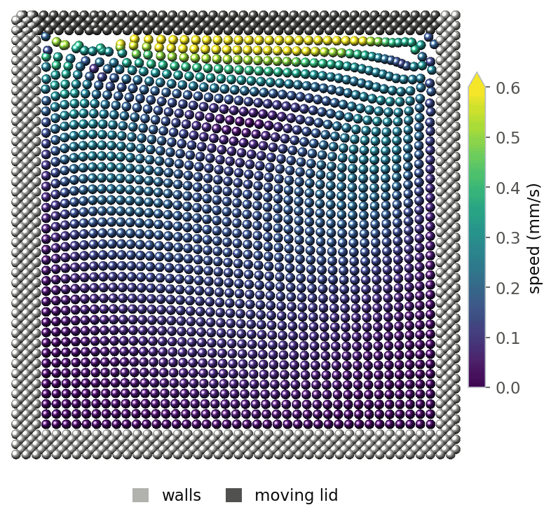
_images/sph-cavity-flow.png — Shear cavity example at the end of the simulation. The fluid particles are colored by their speed, the wall particles are gray, and the moving strip on top is dark gray.

References 

(Hoover2006) Hoover, Smooth Particle Applied Mechanics: The State of the Art, World Scientific, Singapore (2006).

(Liu and Liu) Liu and Liu, Smoothed Particle Hydrodynamics: A Meshfree Particle Method, World Scientific, Singapore (2003).

(Monaghan) Monaghan and Gingold, J Comput Phys, 52, 374-389 (1983).

(Gonzalez) Gonzalez, Sanchez, Macia, Souto-Iglesias, Analysis of WCSPH laminar viscosity models, 4th international SPHERIC workshop, Nantes, France (2009).

(Morris) Morris, Fox, Zhu, J Comput Phys, 136, 214-226 (1997).

(Lucy) Lucy, Astronomical Journal, 82, 1013-1024 (1977).

(Ree) Ree, J Chem Phys, 73, 5401 (1980).

(Gomez-Gesteira) Gomez-Gesteira, Rogers, Dalrymple, Crespo, J Hydraulic Res, 48, 6-27 (2010).