10.5.14. Smoothed Mach dynamics (MACHDYN)
written by Georg C. Ganzenmueller in 2015; converted from
MACHDYN_LAMMPS_userguide.pdf to reStructuredText and updated for
current LAMMPS by Axel Kohlmeyer in 2026
The MACHDYN package implements Smooth Mach Dynamics
(SMD), a meshless method for solving problems in continuum mechanics of
solids and fluids based on smoothed particle hydrodynamics (SPH). This Howto gives an introduction to the methods used,
explains how to set up SMD simulations in LAMMPS, describes the
available material models, and discusses the example inputs in the
examples/PACKAGES/machdyn folder.
Overview
Smoothed particle hydrodynamics was first developed by Lucy (Lucy) and by Gingold and Monaghan (Gingold) to simulate the formation of stars. SPH approximates continuous fields by kernel functions centered at particles that carry the physical properties of the system, e.g. mass, internal energy, or velocity. When applied to fluid flow or the deformation of solids, the partial differential equations of continuum mechanics turn into simple algebraic equations for the particles. As no computational grid is used, SPH can handle arbitrarily large deformations and fracture much more easily than mesh-based methods like the finite element method (FEM), which require well-shaped mesh cells. Applications include impact, explosions, or machining.
The application of SPH to fluids with free surfaces has been very successful, but the simulation of solids with SPH is plagued by numerical instabilities. The interaction of the kernel function with tensile stress results in nonphysical clumping of particles, the so-called tensile instability (Swegle). Belytschko et al. (Belytschko) showed that this instability is caused by the combination of an Eulerian kernel function (particles move in and out of the kernel range of a particle) with the Lagrangian motion of the particles, and that it is absent in a total Lagrangian formulation, where the kernel functions are evaluated in the undeformed reference configuration of the material. A second source of instability remains: since SPH evaluates the field equations only at the particle positions, the solution can contain zero-energy modes of deformation, similar to the hourglass modes of FEM elements with reduced integration. The MACHDYN package controls these modes with an algorithm adapted from FEM (Ganzenmueller), which makes the total Lagrangian SPH formulation stable for large deformations of solids.
The MACHDYN package provides:
the atom style smd, which stores the per-particle data such as volume, mass, kernel radius, contact radius, reference coordinates, stress, and internal energy,
the pair style smd/tlsph for the total Lagrangian SPH formulation (TLSPH), which is best suited for solids,
the pair style smd/ulsph for the updated Lagrangian SPH formulation (ULSPH), which is best suited for fluids and arbitrarily large deformations,
the contact pair styles smd/hertz and smd/tri_surface, which prevent separate bodies from interpenetrating each other or a rigid wall,
a set of material models: equations of state, material strength models, failure models, and viscosity, which are selected with keywords of the pair_coeff command,
the time integration fixes smd/integrate_tlsph and smd/integrate_ulsph and the adaptive time step fix smd/adjust_dt,
rigid walls read from STL files with fix smd/wall_surface, which can be moved with fix smd/move_tri_surf, and velocity boundary conditions with fix smd/setvel,
many computes for output of the per-particle quantities, see below.
The related SPH package implements traditional SPH for fluids, see the Howto sph page.
Quick start
The MACHDYN package is an optional package that requires the Eigen3 library for linear algebra. The MACHDYN section of the Build extras page explains how to compile LAMMPS with this package.
The following input is taken from the rubber_strip_pull example. It
pulls a 2d strip of a linear elastic material apart at two opposite
edges, i.e. it performs a quasi-static tensile test:
# unit system: GPa / mm / ms
variable        E equal 1.0     # Young's modulus
variable        nu equal 0.3    # Poisson ratio
variable        rho equal 1     # initial mass density
variable        q1 equal 0.06   # artificial viscosity, linear coefficient
variable        q2 equal 0.0    # artificial viscosity, quadratic coefficient
variable        hg equal 10.0   # hourglass control coefficient
variable        cp equal 1.0    # ignored

dimension       2
units           si
boundary        sm sm p
atom_style      smd
atom_modify     map array
comm_modify     vel yes
neigh_modify    every 10 delay 0 check yes
newton          off

variable        l0 equal 1.0    # lattice spacing for creating particles
lattice         sq ${l0}
region          box block -10 10 -10 10 -0.1 0.1 units box
create_box      1 box
create_atoms    1 box
group           tlsph type 1

variable        h equal 2.01*${l0}      # SPH kernel range
variable        vol_one equal ${l0}^2   # particle volume for unit thickness
neighbor        ${h} bin
set             group all volume ${vol_one}
set             group all smd/mass/density ${rho}
set             group all diameter ${h}

# velocity boundary conditions
variable        vel0 equal 0.005
region          top block EDGE EDGE 9.0 EDGE EDGE EDGE units box
region          bot block EDGE EDGE EDGE -9.1 EDGE EDGE units box
group           top region top
group           bot region bot
variable        vel_up equal ${vel0}*(1.0-exp(-0.01*time))
variable        vel_down equal -v_vel_up
fix             veltop_fix top smd/setvel 0 v_vel_up 0
fix             velbot_fix bot smd/setvel 0 v_vel_down 0

# material model
pair_style      smd/tlsph
pair_coeff      1 1 *COMMON ${rho} ${E} ${nu} ${q1} ${q2} ${hg} ${cp} &
                *STRENGTH_LINEAR &
                *EOS_LINEAR &
                *END

# time integration with adaptive time step
fix             dtfix tlsph smd/adjust_dt 0.1
fix             integration_fix tlsph smd/integrate_tlsph

# output
compute         S all smd/tlsph/stress
compute         E all smd/tlsph/strain
compute         nn all smd/tlsph/num/neighs
dump            dump_id all custom 10 dump.LAMMPS id type x y z vx vy vz &
                c_S[1] c_S[2] c_S[4] c_nn c_E[1] c_E[2] c_E[4]

variable        stress equal 0.5*(f_velbot_fix[2]-f_veltop_fix[2])/20
variable        length equal xcm(top,y)-xcm(bot,y)
variable        strain equal (v_length-${length})/${length}
fix             stress_curve all print 10 "${strain} ${stress}" file stress_strain.dat screen no
thermo          100
thermo_style    custom step dt f_dtfix v_strain
run             2500
Some notes on this input:
The MACHDYN package contains no hard-coded physical constants, so any consistent system of units can be used. The si setting of the units command only determines the units LAMMPS uses for its output; here, GPa, mm, and ms are used instead of the SI units Pa, m, and s. In this unit system, masses are in kg and densities in kg/mm3.
The atom style smd is required. The pair style smd/tlsph requires an atom map (set with atom_modify), the newton setting off, and that all its particles are members of a group named tlsph. All MACHDYN examples also use comm_modify vel yes, so that ghost particles carry velocities.
The particles are created on a square lattice. Each particle needs a volume, a mass (here computed from the volume and the mass density), and a kernel range h, which is set with the diameter keyword of the set command. The particle volumes must add up to the volume of the simulated body; in 2d, a thickness of one length unit is assumed.
The top and bottom rows of particles are moved apart with a velocity that is smoothly ramped up from zero to avoid a shock wave.
The *COMMON keyword of the pair_coeff command sets the reference density, Young’s modulus, Poisson ratio, and the artificial viscosity and hourglass control coefficients; its last argument is ignored. The keywords that follow select the material model: here, linear elasticity is obtained by combining a linear model for the deviatoric (shear) stress with a linear equation of state for the pressure.
The time step is adjusted every step by fix smd/adjust_dt to 0.1 times the stable time step from the CFL criterion. The fix also outputs the elapsed time.
The engineering stress and strain are computed from the force on the top and bottom rows and from their distance.
The final state of this simulation and the resulting stress-strain curve are shown in the examples section below.
Total Lagrangian formulation
In the total Lagrangian formulation, the conservation and constitutive equations are expressed in terms of the reference coordinates \(\mathbf{X}\) of the initial, undeformed configuration. A mapping \(\mathbf{x} = \varphi(\mathbf{X}, t)\) describes the motion of the body, where \(\mathbf{x}\) are the current coordinates. The displacement is \(\mathbf{u} = \mathbf{x} - \mathbf{X}\). The conservation equations for mass, momentum, and energy are
where \(\rho\) is the mass density, \(\mathbf{P}\) is the first Piola-Kirchhoff stress tensor, and e is the internal energy per unit mass. The subscript 0 indicates that a quantity is evaluated in the reference configuration. J is the determinant of the deformation gradient
which describes the rotation and stretch of a line element from the reference configuration to the current configuration.
SPH approximation and first-order completeness
The SPH approximation of a function f and its gradient in terms of the reference coordinates is
where \(V_j^0\) is the volume of particle j in the reference configuration and the sums run over all neighbors within the kernel range in the reference configuration. Subtracting \(f(\mathbf{X}_i)\) in the gradient expression makes the approximation exact for constant fields (zeroth-order completeness), even for irregular particle arrangements. To also reproduce linear fields exactly (first-order completeness), the kernel gradient is corrected with a correction matrix \(\mathbf{L}_i\) (Bonet):
Deformation gradient and stress update
The deformation gradient and its time derivative follow from the corrected SPH derivatives of the displacement and velocity fields:
The material models in the MACHDYN package are formulated in terms of rates, i.e. they relate a strain rate to a rate of the Cauchy stress, which is then integrated in time. This allows handling non-linear material behavior such as plasticity or damage. To avoid errors due to finite rotations (the stress rate is not objective), the stress rate is integrated in an unrotated frame (Taylor). From the velocity gradient \(\mathbf{L} = \dot{\mathbf{F}} \mathbf{F}^{-1}\), the rate of deformation tensor \(\mathbf{D} = \frac{1}{2}(\mathbf{L} + \mathbf{L}^T)\) is computed. The rotation \(\mathbf{R}\) is obtained from the polar decomposition \(\mathbf{F} = \mathbf{R}\mathbf{U}\), and the unrotated rate of deformation \(\mathbf{d} = \mathbf{R}^T \mathbf{D} \mathbf{R}\) is passed to the material model, which returns the rate of the unrotated stress \(\dot{\boldsymbol{\sigma}}^u\). For linear elasticity with the Lame parameters \(\lambda\) and \(\mu\), for example, \(\dot{\boldsymbol{\sigma}}^u = \lambda\, \text{tr}(\mathbf{d})\, \mathbf{I} + 2 \mu \mathbf{d}\). After the time integration of the unrotated stress, the Cauchy stress is rotated back into the current configuration, \(\boldsymbol{\sigma} = \mathbf{R} \boldsymbol{\sigma}^u \mathbf{R}^T\), and converted to the first Piola-Kirchhoff stress \(\mathbf{P} = J \boldsymbol{\sigma} \mathbf{F}^{-T}\), which links the stress in the current configuration to the reference configuration.
Forces
The forces on the particles are obtained from an SPH approximation of the divergence of the stress. The expression used in the MACHDYN package includes the corrected kernel gradients and is antisymmetric with respect to the exchange of particles i and j, so that the total linear momentum is conserved exactly:
To these forces, an artificial viscosity with a linear (\(Q_1\)) and a quadratic (\(Q_2\)) term is added, which damps high-frequency oscillations and stabilizes shock waves, as well as the hourglass control forces discussed next.
Hourglass control
For each pair of particles, the deformation gradient predicts where particle j should be located relative to particle i. The deviation of the actual distance vector from this prediction,
is the hourglass error vector of this pair. It is zero for any linear deformation and nonzero for the zero-energy (hourglass) modes that cannot be detected by the stress evaluation. The MACHDYN package applies a penalty force along the pair distance vector that is proportional to the projection of \(\boldsymbol{\gamma}_{ij}\) onto the pair distance vector, to the hourglass control coefficient hg, and to Young’s modulus (Ganzenmueller). For particles that are deformed plastically, a viscous form of this force is used instead. Values of hg between about 1 and 20 are recommended. The kernel-weighted average of the hourglass errors of the pairs of a particle can be monitored with compute smd/hourglass/error.
Updating the reference configuration
The total Lagrangian formulation is well suited for elastic deformations with large strains, where the neighbor relations of the material points do not change. For plastic flow, however, the neighbor relations change and the reference configuration has to be updated from time to time. By default, the reference configuration is never updated. With the *UPDATE_CONSTANT or *UPDATE_PAIRWISE arguments of the pair_style smd/tlsph command, an update is triggered when the change of the distance between any pair of particles relative to the reference configuration exceeds a given length or a given fraction of the kernel range, respectively. During an update, the reference coordinates are reset to the current coordinates, the deformation gradient is reset to the identity matrix, and the particle volumes are recomputed from the particle masses and the current densities. Particles with fewer than 15 neighbors also get their kernel range increased by 20%. The stress state is preserved, so the material keeps its memory of the deformation, but strain measures computed after an update refer to the updated reference configuration.
Updated Lagrangian formulation
The pair style smd/ulsph implements an updated Lagrangian formulation, which does away with the reference configuration and evaluates all SPH sums in the current configuration. The particles interacting with a given particle thus change during a simulation, which allows arbitrarily large deformations as in fluid flow. The velocity gradient is computed from SPH derivatives of the velocity field, either plain or with the first-order correction discussed above. The density of each particle is either computed by kernel summation or integrated in time from the trace of the rate of deformation tensor (continuity equation), which in turn determines the pressure from the equation of state. The deviatoric stress is computed from a viscosity model for fluids or integrated in time from a material strength model (using the objective Jaumann stress rate) for solids. The three required arguments of the pair style select between these options:
*DENSITY_SUMMATION or *DENSITY_CONTINUITY: recompute the density every step by kernel summation or integrate it in time. Continuity is more accurate near free surfaces.
*VELOCITY_GRADIENT or *NO_VELOCITY_GRADIENT: whether to compute the velocity gradient. It is required for density continuity and for viscosity and strength models, so it can only be omitted for inviscid fluids with density summation.
*GRADIENT_CORRECTION or *NO_GRADIENT_CORRECTION: whether to apply the first-order correction to the kernel gradients.
Note
The kernel gradient correction makes the method more accurate, but it can lead to severe numerical instabilities when the neighborhood of a particle is ill-defined, i.e. when there are too few neighbors or when they are arranged on a plane or a line. The correction requires the inversion of the matrix \(\mathbf{L}_i\), which then becomes singular. If an updated Lagrangian simulation becomes unstable, try using *NO_GRADIENT_CORRECTION, which is recommended for general fluid simulations.
Since updated Lagrangian SPH suffers from the tensile instability, the *ARTIFICIAL_PRESSURE and *ARTIFICIAL_STRESS keywords of the pair_coeff command can add Monaghan’s artificial pressure or artificial stress terms (Monaghan2000), which counteract the clumping of particles. With fix smd/integrate_ulsph, the kernel range of each particle can be adjusted dynamically so that the number of neighbors stays within a given range.
Setting up a simulation
Per-particle data and initialization
The atom style smd is required for SMD particles. The following per-particle properties must be set consistently:
the volume, with the volume keyword of the set command. The volumes of all particles must add up to the volume of the simulated body, which can be checked with compute smd/vol.
the mass, either directly with the mass keyword of the set command or computed from an already set volume with the smd/mass/density keyword.
the kernel range h, with the diameter keyword of the set command. Please note that the value given to diameter is the range of the SPH kernel function, i.e. the cutoff of the SPH interactions. It is stored as the particle radius h/2, which is output by dump custom with the radius keyword. The examples use a kernel range of 2 to 2.5 times the particle spacing.
the contact radius for the contact pair styles with the smd/contact/radius keyword of the set command. It is typically set to half the particle spacing.
optionally, an initial internal energy with the sph/e keyword of the set command.
Simple geometries can be created with the lattice, region, and create_atoms commands. Complex geometries can be read from a data file with the read_data command, which also sets the volume, mass, kernel radius (i.e. h/2), and contact radius of each particle; the format of a line in the Atoms section is given on the read_data page. The reference coordinates are always initialized with the current coordinates.
Pair styles and their combination
The pair style smd/tlsph is more accurate for solids, while smd/ulsph is better suited for fluids, where arbitrarily large deformations must be described. Both can be used in the same simulation with pair_style hybrid/overlay for different particle types, as shown in the fluid-structure interaction example below. The pair styles have some requirements:
smd/tlsph parameters can only be given for pairs of the same type (i = j), i.e. there are no TLSPH interactions between different particle types. All smd/tlsph particles must be in a group named tlsph, and the pair style requires an atom map and the newton setting off.
smd/ulsph interactions between different particle types are possible, but must be requested with the *CROSS keyword after the parameters for both types have been set.
separate bodies interact only through the contact pair styles smd/hertz (particle-particle) and smd/tri_surface (particle-wall).
Contact forces
The pair style smd/hertz prevents separate physical bodies, e.g. two solid bodies or a solid body and a fluid, from penetrating each other. It can also be used for particles of the same type to model self-contact, e.g. when a flexible part bends and touches itself. The Hertzian contact force between two particles with contact radii \(R_i\) and \(R_j\) at distance r is
for \(r < R_i + R_j\), where E is the contact stiffness given to the pair_coeff command, which has units of pressure. A good choice for the contact stiffness is about 0.1 to 0.5 times the stiffness of the interacting materials, i.e. Young’s modulus of a solid or the bulk modulus of a fluid. Much larger values lead to instabilities with the time step from fix smd/adjust_dt, and much smaller values allow penetration. The contact radii are scaled with the scale_factor argument of the pair style. If the contact radius is half the particle spacing, a scale factor of 1.5 gives a smoother effective contact surface than 1.0. For particles of the same type, an additional check is performed: the contact distance of particles that were within each other’s kernel range in the reference configuration is reduced to half of \(R_i + R_j\). Thus, self-contact forces mostly act between particles that do not already interact through the SPH pair style.
Material models
The material models of the MACHDYN package decompose the Cauchy stress into an isotropic pressure p and a deviatoric (shear) stress \(\boldsymbol{\sigma}_d\),
The pressure is computed by an equation of state (EOS) from the volumetric deformation, and the deviatoric stress by a material strength model for solids or a viscosity model for fluids. The models are selected independently with keywords of the pair_coeff command following the mandatory *COMMON keyword. The syntax of all keywords is given on the pair_style smd/tlsph and pair_style smd/ulsph pages. The following table lists the available models:
Keyword |
smd/tlsph |
smd/ulsph |
|---|---|---|
*EOS_NONE |
yes |
no |
*EOS_LINEAR |
yes |
yes |
*EOS_SHOCK |
yes |
no |
*EOS_POLYNOMIAL |
yes |
no |
*EOS_TAIT |
no |
yes |
*EOS_PERFECT_GAS |
no |
yes |
*STRENGTH_LINEAR |
yes |
yes |
*STRENGTH_LINEAR_PLASTIC |
yes |
yes |
*JOHNSON_COOK |
yes |
no |
*VISCOSITY_NEWTON |
no |
yes |
*FAILURE_MAX_PLASTIC_STRAIN |
yes |
no |
*FAILURE_MAX_PAIRWISE_STRAIN |
yes |
no |
*FAILURE_ENERGY_RELEASE_RATE |
yes |
no |
*ARTIFICIAL_PRESSURE, *ARTIFICIAL_STRESS |
no |
yes |
Several elastic constants are derived from the *COMMON parameters. For smd/tlsph, Young’s modulus E and Poisson ratio \(\nu\) give the shear modulus \(G = E/(2(1+\nu))\), the Lame parameter \(\lambda = E\nu/((1+\nu)(1-2\nu))\), the bulk modulus \(K = \lambda + 2G/3\), and the speed of sound \(c_0 = \sqrt{(\lambda + 2G)/\rho_0}\). For smd/ulsph, the bulk modulus is computed from the reference speed of sound and density, \(K = c_0^2 \rho_0\).
Equations of state
In the following, \(\mu = \rho/\rho_0 - 1\) is the volume change, e the internal energy per unit mass, and \(e_0 = 0\) its value at the beginning of the simulation.
*EOS_LINEAR: linear relation between pressure and volume change, \(p = K\mu\). For smd/tlsph, it is implemented in rate form, \(\dot p = -K\,\text{tr}(\mathbf{d})\), which is equivalent for small deformations.
*EOS_SHOCK c0 S \(\Gamma\): Mie-Grueneisen equation of state with a linear relation \(U_s = c_0 + S u_p\) between the shock velocity and the particle velocity,
\[p_H = \frac{\rho_0 c_0^2 \mu (1 + \mu)}{\left[1 - (S - 1)\mu\right]^2}, \qquad p = p_H + \rho\,\Gamma\,(e - e_0)\]*EOS_POLYNOMIAL C0 … C3: polynomial equation of state. The pressure is \(p = C_0 + C_1\mu + C_2\mu^2 + C_3\mu^3\) for compression (\(\mu > 0\)) and \(p = C_0 + C_1\mu + C_3\mu^3\) for expansion.
*EOS_TAIT n: Tait equation of state \(p = \frac{\rho_0 c_0^2}{n}\left[ (\rho/\rho_0)^n - 1 \right]\), which neglects thermal effects. A typical value for water is n = 7.
*EOS_PERFECT_GAS \(\gamma\): ideal gas, \(p = (\gamma - 1)\rho e\), with the heat capacity ratio \(\gamma\).
Material strength and viscosity models
*STRENGTH_LINEAR: deviatoric part of linear (Hookean) elasticity, \(\dot{\boldsymbol{\sigma}}_d = 2G\mathbf{d}_d\), where \(\mathbf{d}_d\) is the deviatoric part of the rate of deformation. For smd/tlsph, the shear modulus is derived from the *COMMON parameters; for smd/ulsph, it is given as an argument.
*STRENGTH_LINEAR_PLASTIC: linear elastic / plastic material with linear hardening. At each time step, an elastic trial update of the deviatoric stress is performed. If the von Mises equivalent stress of the trial stress exceeds the yield stress \(\sigma_y = \sigma_{y,0} + H \varepsilon_p\), where \(\varepsilon_p\) is the equivalent plastic strain and H the hardening parameter, the deviatoric stress is scaled back to the yield surface (radial return algorithm (Bower)). The increase of the plastic strain can be output with compute smd/plastic/strain.
*JOHNSON_COOK A B a C \(\dot\varepsilon_0\): Johnson-Cook strength model for ductile metals (Johnson). The update is the same as for the linear plastic model, but the yield stress depends on the equivalent plastic strain and plastic strain rate:
\[\sigma_y = \left( A + B \varepsilon_p^a \right) \left( 1 + C \ln \frac{\dot\varepsilon_p}{\dot\varepsilon_0} \right)\]where the ratio of the strain rates is limited to values of at least 1. The thermal softening of the original model is not included.
*VISCOSITY_NEWTON \(\mu\): Newtonian fluid with dynamic viscosity \(\mu\), \(\boldsymbol{\sigma}_d = 2\mu\mathbf{d}_d\). This model cannot be combined with a strength model.
Damage and failure models
Classical continuum mechanics failure models act on an integration point, i.e. a particle, and degrade the stress it can carry. An alternative approach, which is in much better agreement with the meshless nature of SPH, degrades only the interactions between specific pairs of particles. This approach is similar to the visibility criterion used in other meshless methods (Belytschko2) and to bond breaking in peridynamics, see the Howto peri page. All failure models of the MACHDYN package degrade pairwise interactions with smd/tlsph. The pairwise strain of particles i and j is \(\varepsilon_{ij} = (r - r_0)/r_0\), where r and \(r_0\) are the current and reference distances. The pairwise damage \(d_{ij}\) scales the interaction by \(1 - d_{ij}\), and the interaction is permanently removed when \(d_{ij}\) reaches 1. Since damage requires a positive pairwise strain, failure can only occur under tension or shear, but not under compression.
*FAILURE_MAX_PAIRWISE_STRAIN \(\varepsilon_\text{max}\): the pairwise damage is \(d_{ij} = (\varepsilon_{ij} - \varepsilon_\text{max})/(2\varepsilon_\text{max})\) for \(\varepsilon_{ij} > \varepsilon_\text{max}\), and zero otherwise. The damage is reversible until the interaction is removed. This model is numerically much more stable than the plastic strain based model and cannot be combined with updates of the reference configuration.
*FAILURE_MAX_PLASTIC_STRAIN \(\varepsilon_{p,\text{max}}\): when the equivalent plastic strain of a particle exceeds the threshold, its damage variable is set to 1. When both particles of a pair are damaged, the pairwise strain at that moment is stored as the onset strain \(\varepsilon_{ij,0}\), and the pairwise damage is then \(d_{ij} = (\varepsilon_{ij} - \varepsilon_{ij,0})/(2\varepsilon_{ij,0})\). The per-particle damage can be output with compute smd/damage. This model can lead to severe instabilities under compression.
*FAILURE_ENERGY_RELEASE_RATE \(G_c\): the work done by the stress forces of each pair is accumulated, and the interaction is removed when the work per volume exceeds a threshold derived from the critical energy release rate \(G_c\) (energy per area). The conversion assumes a 2d plane strain geometry.
Boundary conditions
Dirichlet boundary conditions can be imposed directly on particles with fix smd/setvel for velocities, as in the quick start example above, or with fix setforce for forces. Particles that are not integrated in time, because they are not in the group of an integration fix, never move, which is equivalent to a fixed displacement boundary condition. Such particles can form a container, as in the fluid-structure interaction example below.
Rigid walls with complex shapes can be read from triangulated surfaces
in STL format with fix smd/wall_surface.
The fix creates one particle for each triangle, and the pair style
smd/tri_surface computes contact
forces between the SPH particles and these triangles. Directly after
the fix command, a run 0 command is required to properly
register the new particles. The walls can be moved with fix
smd/move_tri_surf. The current
coordinates of the triangles can be output with compute
smd/triangle/vertices and dump
custom and converted to VTK format with the dump2vtk_tris
program from the smd tool. The walls can also be included
in images created with dump image. See the funnel
flow example below.
Time integration and stable time step
Particles interacting with smd/tlsph must be integrated with fix smd/integrate_tlsph and particles interacting with smd/ulsph with fix smd/integrate_ulsph. Both use the velocity-Verlet algorithm for positions and velocities and also integrate the internal energy; smd/integrate_ulsph also updates the particle volumes and can adjust the kernel ranges. Both fixes can limit the velocity of particles, which destroys the conservation of energy, but can help to deal with instabilities.
For any explicit time integration scheme, the time step \(\Delta t\) must satisfy the Courant-Friedrichs-Lewy (CFL) criterion \(\Delta t < h/c_0\), where h is a characteristic distance between integration points and \(c_0\) is the speed at which information propagates. For a fluid, this speed is \(c_0 = \sqrt{K/\rho}\) with the bulk modulus K; in a solid, the shear modulus G increases it to \(c_0 = \sqrt{(K + 4G/3)/\rho}\). For non-linear material models, the effective moduli change during a simulation. Fix smd/adjust_dt computes the stable time step for each particle from the current effective moduli and also considers the stable time steps of the contact pair styles. The time step is set to the smallest of these values multiplied with a safety factor, typically 0.1. The fix outputs the elapsed simulated time, which is otherwise not easily available with a variable time step.
Output of particle quantities
Some per-particle quantities can be output directly with dump custom, e.g. the particle mass (mass) and half of the kernel range (radius). Many more are available through the following computes:
Compute |
Quantity |
|---|---|
particle volume |
|
mass density |
|
contact radius |
|
internal energy |
|
damage variable |
|
equivalent plastic strain (TLSPH) |
|
equivalent plastic strain rate (TLSPH) |
|
hourglass error (TLSPH) |
|
Cauchy stress tensor and von Mises equivalent stress |
|
strain tensor |
|
strain rate tensor |
|
deformation gradient (TLSPH) |
|
deformed particle shape as an ellipsoid (TLSPH) |
|
stable time step of each particle (TLSPH) |
|
number of neighbors within the kernel range |
|
effective shear modulus (ULSPH) |
|
coordinates of the triangles of walls from STL files |
The per-particle vectors can be summed up for thermodynamic output with compute reduce, e.g. to monitor the total internal energy.
Examples
The following examples are included in the examples/PACKAGES/machdyn
folder. Most of the inputs run only a small number of time steps by
default, so that they can be used for regression testing. The number of
steps is then set by the index style variable nsteps, which can be
changed with the -var command-line switch, e.g.
lmp -in in.aluminum_strip_pull -var nsteps 30000. The README file
in the folder lists the values needed for the complete examples, which
were used for the figures below.
Tensile loading of a rubber strip
The input rubber_strip_pull/in.rubber_strip_pull is discussed in
the quick start section above. It illustrates
the basic features of total Lagrangian SPH. Due to the Poisson effect,
the material contracts laterally and a non-homogeneous distribution of
stress develops. For 2d plane strain conditions, the effective Young’s
modulus is \(E_\text{2d} = E/(1 - \nu^2) \approx 1.1\) GPa. This
value is well reproduced by the slope of the stress-strain curve, at
least for small strains. At larger strains, deviations are expected,
because the engineering stress used in the input is no longer a good
measure. The folder also contains a gnuplot script for plotting the
stress-strain curve.
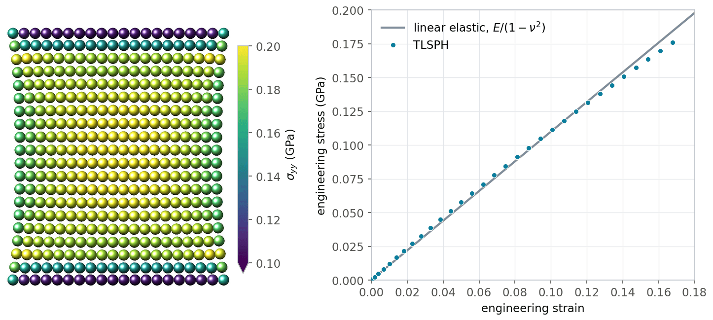
Rubber strip example. Left: particles at the end of the simulation colored by the yy component of the stress. Right: stress-strain curve compared to the linear elastic plane strain relation.
Tensile loading of an aluminum strip
The input aluminum_strip_pull/in.aluminum_strip_pull illustrates the
modeling of a real material, here aluminum, with a complex material
model including failure. The setup is the same as for the rubber strip,
but the material is described by the polynomial equation of state, the
Johnson-Cook strength model, and the maximum plastic strain failure
model:
pair_style      smd/tlsph
pair_coeff      1 1 *COMMON ${rho} ${E} ${nu} ${q1} ${q2} ${hg} ${cp} &
                *EOS_POLYNOMIAL ${eosC0} ${eosC1} ${eosC2} ${eosC3} ${eosC4} ${eosC5} ${eosC6} &
                *JOHNSON_COOK ${JC_A} ${JC_B} ${JC_N} ${JC_C} ${JC_epsdot0} ${Troom} ${Tmelt} ${JC_M} &
                *FAILURE_MAX_PLASTIC_STRAIN 1.2 &
                *END
By default, the example input runs only 2000 steps, which reaches an
engineering strain of about 1.3%, i.e. it covers the elastic regime and
the onset of plastic yielding, when the von Mises stress reaches the
initial yield stress A = 0.324 GPa. The figure below was obtained by
running 30000 steps (-var nsteps 30000). The strip yields and
hardens, then necks, and finally fails when the plastic strain in the
neck exceeds the failure threshold.
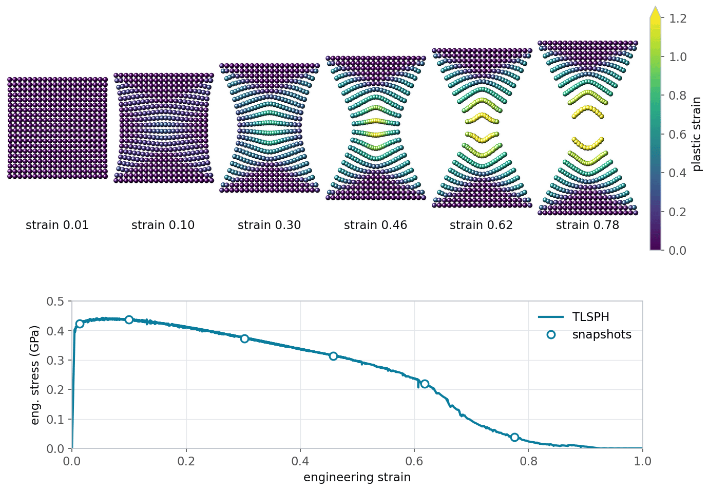
Aluminum strip example run for 30000 steps. Top: particles colored by their equivalent plastic strain at different engineering strains. Bottom: engineering stress-strain curve.
Fluid-structure interaction
The input
fluid_structure_interaction/in.fluid_structure_interaction shows
how a fluid and deformable solids can be coupled. A water column
collapses under gravity in a container and pushes several solid objects
around until the system comes to rest due to viscous damping. The solid
objects have a lower mass density than water and finally float on the
water. Water is modeled with the updated Lagrangian formulation and
the Tait equation of state, while the solid objects are modeled with the
total Lagrangian formulation and a linear elastic / plastic material
model. Contact forces between the container, the solid objects, and the
water prevent their mutual penetration. The particles of the container
are not integrated in time and thus never move.
pair_style      hybrid/overlay smd/ulsph *DENSITY_CONTINUITY *VELOCITY_GRADIENT *NO_GRADIENT_CORRECTION &
                               smd/tlsph smd/hertz ${contact_scale}
pair_coeff      1 1 smd/ulsph *COMMON ${rho_water} ${c0} ${q1} ${Cp} 0 &
                *EOS_TAIT 7.0 &
                *END
pair_coeff      2 2 smd/tlsph *COMMON ${rho_obj} ${E} ${nu} ${q1} ${q2} ${Hg} ${Cp} &
                *STRENGTH_LINEAR_PLASTIC ${sigma_yield} ${hardening_parameter} &
                *EOS_LINEAR &
                *END
pair_coeff      3 3 none
pair_coeff      1 2 smd/hertz ${contact_stiffness}
pair_coeff      1 3 smd/hertz ${contact_stiffness}
pair_coeff      2 3 smd/hertz ${contact_stiffness}
pair_coeff      2 2 smd/hertz ${contact_stiffness}

fix             dtfix tlsph smd/adjust_dt 0.1
fix             integration_fix_water water smd/integrate_ulsph adjust_radius 1.01 10 15
fix             integration_fix_solids solids smd/integrate_tlsph
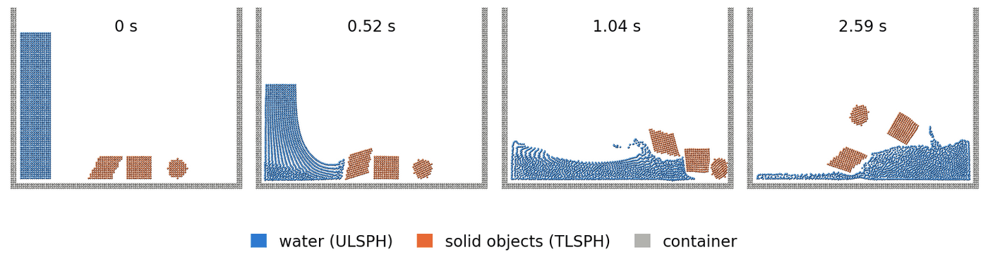
Snapshots of the fluid-structure interaction example (lower part of the container).
Funnel flow
The input funnel_flow/in.funnel_flow simulates the gravity-driven
flow of a fluid through a complex 3d geometry, which is read from the
file boundary.stl. The fluid is modeled with the updated Lagrangian
formulation and the Tait equation of state. The STL geometry acts as a
rigid wall through the smd/tri_surface pair style:
pair_style      hybrid/overlay smd/tri_surface 1.0 &
                smd/ulsph *DENSITY_CONTINUITY *VELOCITY_GRADIENT *NO_GRADIENT_CORRECTION
pair_coeff      1 1 smd/ulsph *COMMON ${rho} ${c0} ${q1} ${cp} ${hg} &
                *EOS_TAIT 2 &
                *END
pair_coeff      2 2 none
pair_coeff      1 2 smd/tri_surface ${contact_stiffness}

fix             stl_surface_fix all smd/wall_surface boundary.stl 2 65535
run             0 # required directly after loading the STL file
group           surface type 2
fix             force_fix surface setforce 0 0 0
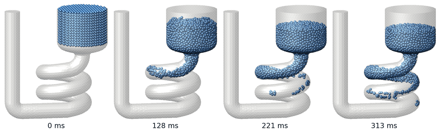
Gravity-driven fluid flow through a complex geometry, rendered with dump image including the wall surface.
A movie of this example is available on the LAMMPS website.
Impact of two rubber rings
In the input rubber_rings_3d/in.rubber_rings_3d, two rings read from
a data file collide with each other. One ring is linear elastic, the
other one is elastic - ideal plastic. Contact forces between the rings
are computed with the smd/hertz pair style. The
elastic ring recovers its shape after the impact, while the plastic ring
is permanently deformed. About three quarters of the initial kinetic
energy is converted into internal energy (deformation work), while the
total energy is conserved to about 0.1%.
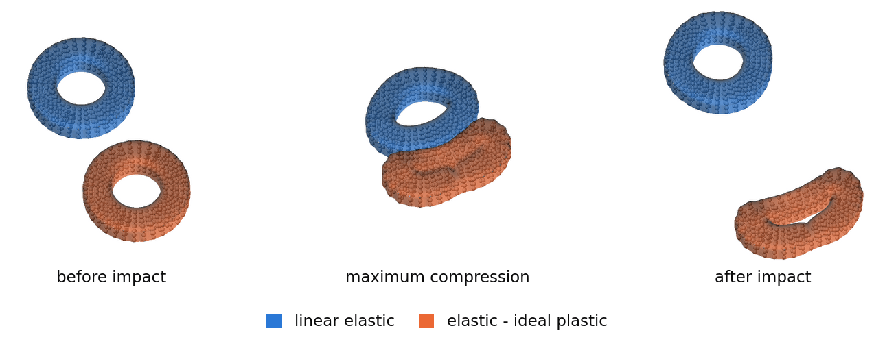
Impact of a linear elastic ring and an elastic - ideal plastic ring. The shape of each ring is shown as a translucent surface computed from the particle positions with fix graphics/isosurface.
The input file contains commented out commands for creating such images with dump image. A movie of this example is available on the LAMMPS website.
References
(Lucy) Lucy, Astronomical Journal, 82, 1013-1024 (1977).
(Gingold) Gingold and Monaghan, Mon Not R Astron Soc, 181, 375-389 (1977).
(Swegle) Swegle, Hicks, Attaway, J Comput Phys, 116, 123-134 (1995).
(Belytschko) Belytschko, Guo, Liu, Xiao, Int J Numer Meth Eng, 48, 1359-1400 (2000).
(Ganzenmueller) Ganzenmueller, Comput Methods Appl Mech Eng, 286, 87-106 (2015).
(Bonet) Bonet and Lok, Comput Methods Appl Mech Eng, 180, 97-115 (1999).
(Taylor) Taylor and Flanagan, PRONTO 2D: A two-dimensional transient solid dynamics program, Sandia report SAND86-0594, Sandia National Laboratories (1987).
(Monaghan2000) Monaghan, J Comput Phys, 159, 290-311 (2000).
(Bower) Bower, Applied Mechanics of Solids, CRC Press (2011).
(Johnson) Johnson and Cook, Proceedings of the 7th International Symposium on Ballistics, 541-547 (1983).
(Belytschko2) Belytschko, Lu, Gu, Int J Numer Meth Eng, 37, 229-256 (1994).