Models for normal contact in granular interactions
The normal force acts along the vector connecting the center of two particles, i.e. normal to the plane of contact between particles. In all cases, the normal force is modeled as a function of overlap \(\delta_{ij}\). The following quantities are common to normal models:
\(\delta_{ij} = R_i + R_j - \|\mathbf{r}_{ij}\|\) is the particle overlap,
\(R_i, R_j\) are the particle radii,
\(\mathbf{r}_{ij} = \mathbf{r}_i - \mathbf{r}_j\) is the vector separating the two particle centers (note the i-j ordering so that the force is positive for repulsion), and
\(\mathbf{n} = \frac{\mathbf{r}_{ij}}{\|\mathbf{r}_{ij}\|}\) is the unit vector along the direction connecting the two particle centers.
\(R_\text{eff} = \frac{R_iR_j}{R_i+R_j}\) is the effective radius for particles i and j, or set to the radius of the particle in a wall-particle contact.
Unless otherwise specified, the radius of the contact region is given by \(\sqrt{\delta R_\text{eff}}\) for all models. Notable exceptions are jkr and epa/nonlinear.
hooke normal model
Parameters: \(k_n\), \(\eta_{n0}\) (or \(e\))
Example:
pair_style granular
pair_coeff * * hooke 1000.0 50.0 tangential linear_nohistory 1.0 0.4 damping mass_velocity
For the hooke model, the normal component of force acting on particle i due to contact with particle j is given by:
The units of the spring constant \(k_n\) are force/distance, or equivalently mass/time2.
hertz normal model
Parameters: \(k_n\), \(\eta_{n0}\) (or \(e\))
Example:
pair_style granular
pair_coeff * * hertz 1000.0 50.0 tangential mindlin 1000.0 1.0 0.4 limit_damping
For the hertz model, the normal force is given by:
The units of the spring constant \(k_n\) are force/length^2, or equivalently pressure.
hertz/material normal model
Parameters: \(E\), \(\eta_{n0}\) (or \(e\)), \(\nu\)
Example:
pair_style granular
pair_coeff * * hertz/material 1.0e8 50.0 0.3 tangential mindlin NULL 1.0 0.4 damping viscoelastic
For the hertz/material model, the normal force is given by:
Here, \(E_{eff} = E = \left(\frac{1-\nu_i^2}{E_i} + \frac{1-\nu_j^2}{E_j}\right)^{-1}\) is the effective Young’s modulus, with \(\nu_i, \nu_j\) the Poisson ratios of the particles of types i and j. Note that if the elastic modulus and the shear modulus of the two particles are the same, the hertz/material model is equivalent to the hertz model with \(k_n = 4/3 E_{eff}\)
dmt normal model
Parameters: \(E\), \(\eta_{n0}\) (or \(e\)), \(\nu\), \(\gamma\)
Example:
pair_style granular
pair_coeff * * dmt 1.0e8 50.0 0.3 0.1 tangential mindlin NULL 1.0 0.4 damping viscoelastic
The dmt model corresponds to the (Derjaguin-Muller-Toporov) cohesive model, where the force is simply Hertz with an additional attractive cohesion term:
jkr normal model
Parameters: \(E\), \(\eta_{n0}\) (or \(e\)), \(\nu\), \(\gamma\)
Example:
pair_style granular
pair_coeff * * jkr 1.0e8 50.0 0.3 0.1 tangential mindlin NULL 1.0 0.4 damping viscoelastic
The jkr model is the (Johnson-Kendall-Roberts) model, where the force is computed as:
Here, \(a\) is the radius of the contact zone, related to the overlap \(\delta\) according to:
LAMMPS internally inverts the equation above to solve for a in terms of \(\delta\), then solves for the force in the previous equation. Additionally, note that the JKR model allows for a tensile force beyond contact (i.e. for \(\delta < 0\)), up to a maximum of \(3\pi\gamma R\) (also known as the ‘pull-off’ force). Note that this is a hysteretic effect, where particles that are not contacting initially will not experience force until they come into contact \(\delta \geq 0\); as they move apart and (\(\delta < 0\)), they experience a tensile force up to \(3\pi\gamma R\), at which point they lose contact.
mdr normal model
Parameters: \(E\), \(\nu\), \(Y\), \(\Delta\gamma\), \(\psi_b\), \(\eta_{n0}\)
Example:
pair_style granular
pair_coeff * * mdr 5e6 0.4 1.9e5 2.0 0.5 0.5 tangential linear_history 940.0 1.0 0.7 rolling sds 2.7e5 0.0 0.6 damping mdr 1
The mdr model is a mechanically-derived contact model designed to capture the contact response between adhesive elastic-plastic particles under large deformation. The theoretical foundations of the mdr model are detailed in the two-part series Zunker and Kamrin Part I and Zunker and Kamrin Part II. Further development and demonstrations of its application to industrially relevant powder compaction processes are presented in Zunker et al.. If you use the mdr normal model the only supported damping option is the mdr damping class described below.
The model requires the following inputs:
1. Young’s modulus \(E > 0\) : The Young’s modulus is commonly reported for various powders.
2. Poisson’s ratio \(0 \le \nu \le 0.5\) : The Poisson’s ratio is commonly reported for various powders.
3. Yield stress \(Y \ge 0\) : The yield stress is often known for powders composed of materials such as metals but may be unreported for ductile organic materials, in which case it can be treated as a free parameter.
4. Effective surface energy \(\Delta\gamma \ge 0\) : The effective surface energy for powder compaction applications is most easily determined through its relation to the more commonly reported critical stress intensity factor \(K_{Ic} = \sqrt{2\Delta\gamma E/(1-\nu^2)}\).
5. Critical confinement ratio \(0 \le \psi_b \le 1\) : The critical confinement ratio is a tunable parameter that determines when the bulk elastic response is triggered. Lower values of \(\psi_b\) delay the onset of the bulk elastic response.
6. Damping coefficient \(\eta_{n0} \ge 0\) : The damping coefficient is a tunable parameter that controls damping in the normal direction.
Note
The values for \(E\), \(\nu\), \(Y\), and \(\Delta\gamma\) (i.e., \(K_{Ic}\)) should be selected for zero porosity to reflect the intrinsic material property rather than the bulk powder property.
The mdr model produces a nonlinear force-displacement response, therefore the critical timestep \(\Delta t\) depends on the inputs and level of deformation. As a conservative starting point the timestep can be assumed to be dictated by the bulk elastic response such that \(\Delta t = 0.08\sqrt{m/k_\textrm{bulk}}\), where \(m\) is the mass of the smallest particle and \(k_\textrm{bulk} = \kappa R_\textrm{min}\) is an effective stiffness related to the bulk elastic response. Here, \(\kappa = E/(3(1-2\nu))\) is the bulk modulus and \(R_\textrm{min}\) is the radius of the smallest particle.
The atom_style must be set to sphere 1 to enable dynamic particle radii. The mdr model is designed to respect the incompressibility of plastic deformation and inherently tracks free surface displacements induced by all particle contacts. In practice, this means that all particles begin with an initial radius, however as compaction occurs and plastic deformation is accumulated, a new enlarged apparent radius is defined to ensure that volume change due to plastic deformation is not lost. This apparent radius is stored as the atom radius meaning it is used for subsequent neighbor list builds and contact detection checks. The advantage of this is that multi-neighbor dependent effects such as formation of secondary contacts caused by radial expansion are captured by the mdr model. Setting atom_style sphere 1 ensures that updates to the particle radii are properly reflected throughout the simulation.
atom_style sphere 1
Newton’s third law must be set to off. This ensures that the neighbor lists are constructed properly for the topological penalty algorithm used to screen for non-physical contacts occurring through obstructing particles, an issue prevalent under large deformation conditions. For more information on this algorithm see Zunker et al..
newton off
The definition of multiple mdr models in the pair_style is currently not supported. Similarly, the mdr model cannot be combined with a different normal model in the pair_style. Physically this means that only one homogeneous collection of particles governed by a single mdr model is allowed.
The mdr model currently only supports fix wall/gran/region, not fix wall/gran. If the mdr model is specified for the pair_style any fix wall/gran/region commands must also use the mdr model. Additionally, the following mdr inputs must match between the pair_style and fix wall/gran/region definitions: \(E\), \(\nu\), \(Y\), \(\psi_b\), and \(\eta_{n0}\). The exception is \(\Delta\gamma\), which may vary, permitting different adhesive behaviors between particle-particle and particle-wall interactions.
Note
The mdr model has a number of custom property/atom and pair/local definitions that can be called in the input file. The useful properties for visualization and analysis are described below.
In addition to contact forces the mdr model also tracks the following quantities for each particle: elastic volume change, average normal stress components, total surface area involved in contact, and individual contact areas. In the input script, these quantities are initialized by calling run 0 and can then be accessed using subsequent compute commands. The last compute command uses pair/local p13 to calculate the pairwise contact areas for each active contact in the group-ID. Due to the use of an apparent radius in the mdr model, the keyword/arg pair cutoff radius must be specified for pair/local to properly detect existing contacts.
run 0
compute ID group-ID property/atom d_Velas
compute ID group-ID property/atom d_sigmaxx
compute ID group-ID property/atom d_sigmayy
compute ID group-ID property/atom d_sigmazz
compute ID group-ID property/atom d_Acon1
compute ID group-ID pair/local p13 cutoff radius
Note
The mdr model has two example input scripts within the examples/granular directory. The first is a die compaction simulation involving 200 particles named in.tableting.200. The second is a triaxial compaction simulation involving 12 particles named in.triaxial.compaction.12.
epa/linear model
Parameters: \(k_1\), \(\eta_{n0}\) (or \(e\)), \(\hat{k}_2\), \(k_c\), \(\phi_f\), \(f_0\)
Example:
pair_style granular
pair_coeff * * epa/linear 1000.0 50.0 5000.0 200.0 0.5 0.0 tangential linear_history 500.0 1.0 0.4 damping mass_velocity
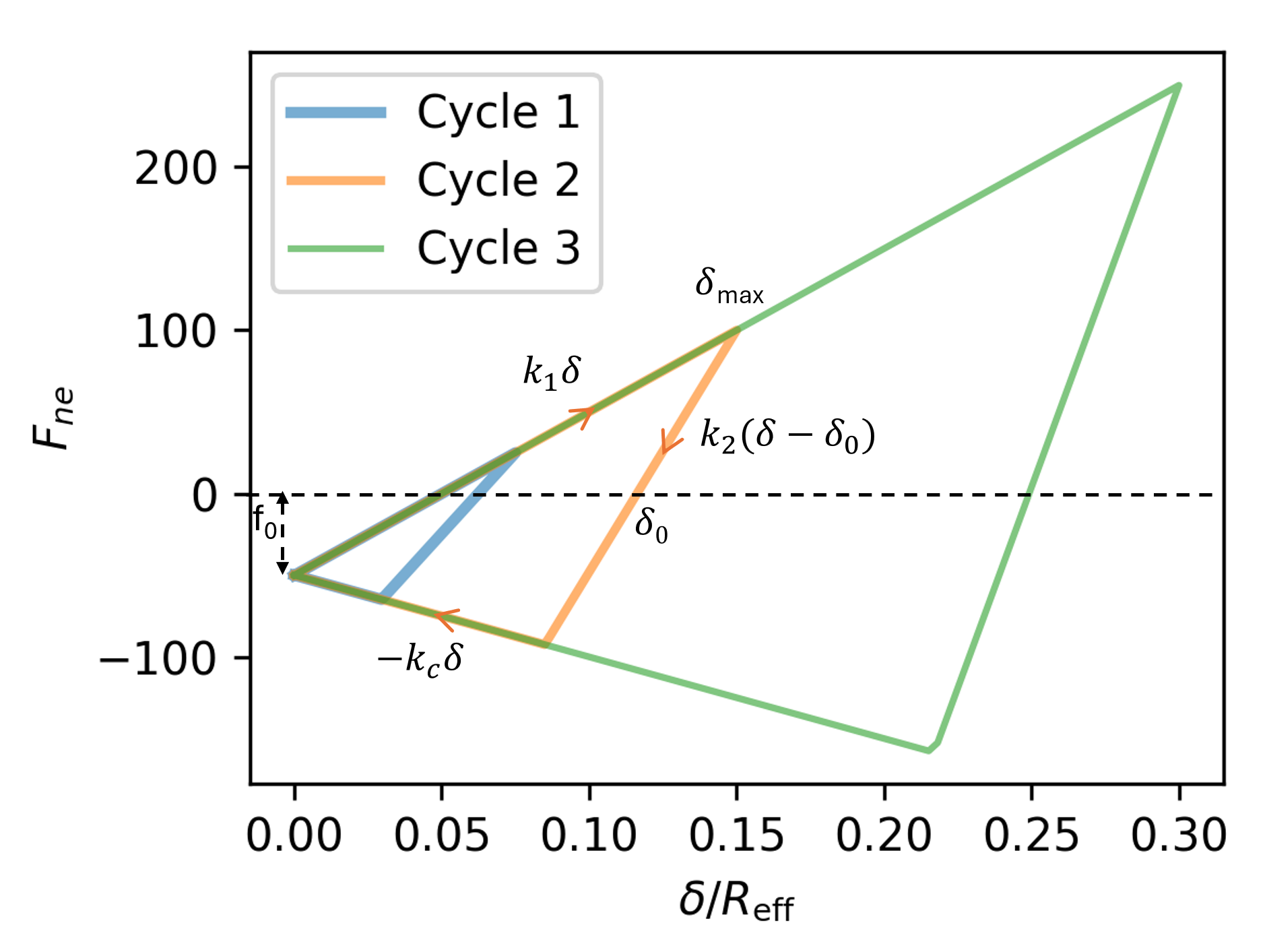
The epa/linear model is the linear elastic-plastic-adhesive model proposed by (Luding), where the force is computed according to:
where
and
Initial loading proceeds along the elastic branch with stiffness \(k_1\). The maximum overlap \(\delta_\text{max}\) is stored and updated throughout the duration of the contact. Unloading takes place with stiffness \(k_2\), which increases with the maximum overlap \(\delta_\text{max}\), up to a maximum value of \(\hat{k_2}\). Re-loading proceeds along the same line of slope \(k_2\), until the overlap \(\delta_\text{max}\) is reached, at which point further loading takes place with slope \(k_1\). Unloading below \(\delta_\text{min} = (k_2-k_1)\delta_\text{max}(k_2+k_c)\) leads to the adhesive branch, where unloading proceeds with stiffness \(k_c\). A constant cohesive force \(f_0\) can optionally also be specified. The overlap at which \(k_2\) reaches its maximum value \(\hat{k_2}\) is determined by a plastic overlap range, specified as a user input \(\phi_f\), with typical values \(0<\phi_f<1\).
The critical force for purposes of computing friction is given by \(F_\text{ne} + f_0\) if not on the adhesive branch, or \(F_\text{ne} + f_0 + k_c\delta\) if on the adhesive branch.
epa/nonlinear model
Example:
pair_style granular
pair_coeff * * epa/nonlinear 1.0e8 50.0 0.3 0.5 0.0 1000.0 1.5 1.0 tangential mindlin NULL 1.0 0.4 damping viscoelastic
- Parameters: \(E\), \(\eta_{n0}\) (or \(e\)), \(\nu\),
\(\lambda_p\), \(f_0\), \(k_{c}\), \(m\), \(n\)
The epa/nonlinear model is very similar to the nonlinear elastic-plastic-adhesive model proposed by Thakur et al, also known as the Edinburgh elasto-plastic adhesive (EEPA) model. The force is computed according to:
where the stiffness can be related to the elastic modulus according to:
Here, \(E_{eff} = E = \left(\frac{1-\nu_i^2}{E_i} + \frac{1-\nu_j^2}{E_j}\right)^{-1}\) is the effective Young’s modulus, with \(\nu_i, \nu_j\) the Poisson ratios of the particles of types i and j, and \(R_\text{eff}\) is the effective radius. The inclusion of the \(R_\text{eff}\) term in the definitions of \(k_1\) and \(k_c\) is not found in the original (Thakur et al) paper, but appears in other formulations of the EEPA model (e.g. (Morrisey thesis)). The exponent \(2-m\) ensures dimensional consistency for varying \(m\) values, while retaining particle radius dependence. For \(m=3/2\), the model recovers the Hertzian limit; for other values of \(m\), the modulus should be treated as a calibrated parameter, since such models do not have a direct connection to material properties.
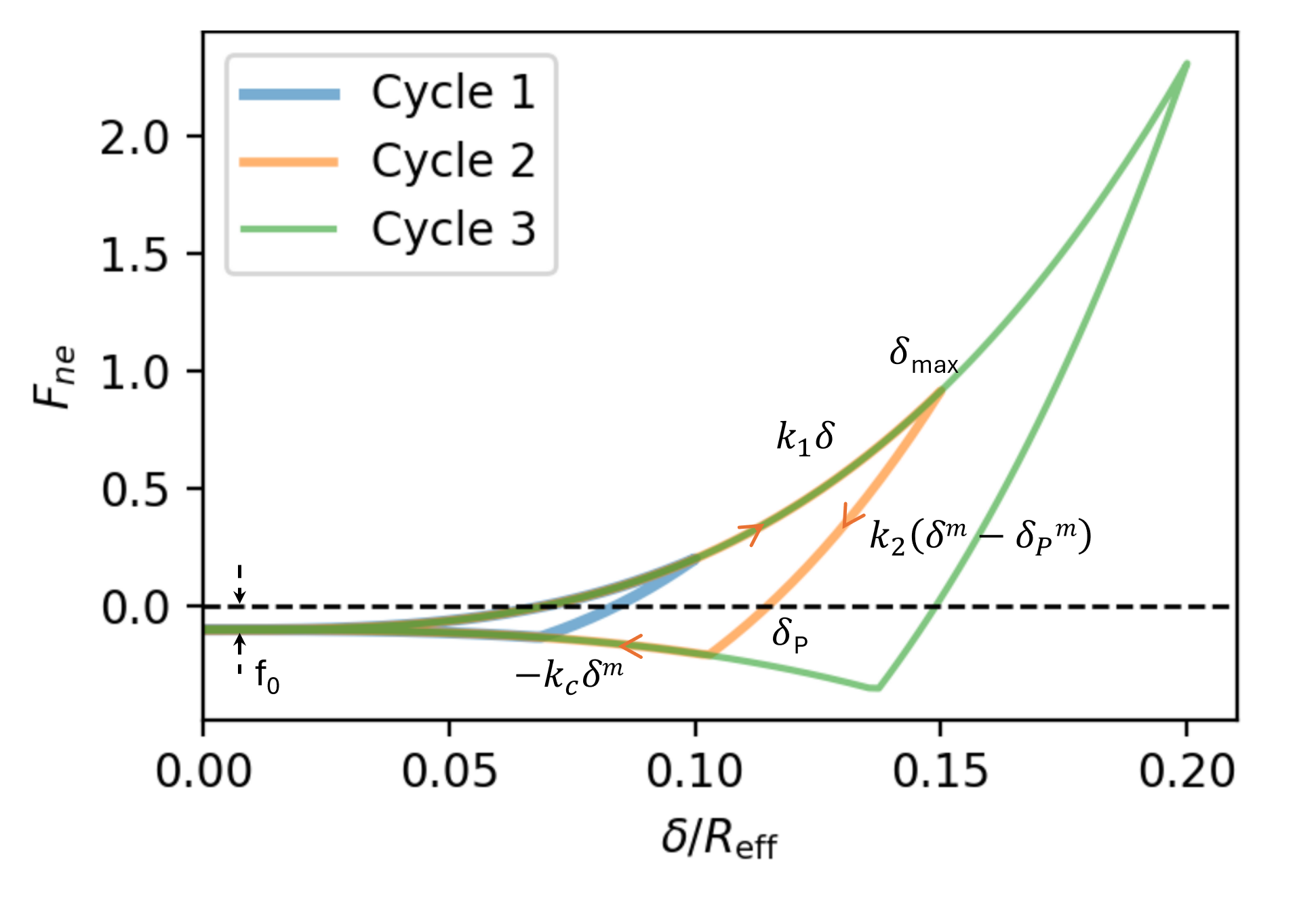
Initial loading proceeds along the \(k_1\delta^m\) branch. The maximum overlap \(\delta_\text{max}\) is stored and updated throughout the duration of the contact. The overlap reference plastic deformation \(\delta_p\) is then given by:
Unloading proceeds along \(k_2(\delta^m-\delta_p^m)\), and re-loading proceeds along the same branch, until \(\delta_\text{max}\) is reached, at which point further loading resumes along \(k_1\delta^m\). If unloading continues such that \(-k_c\delta^n \ge k_2(\delta^m-\delta_p)\), the adhesive branch is activated, where unloading proceeds along \(-k_c\delta^n\). A constant cohesive contact force \(f_0\) can optionally also be specified.
The contact radius is given by \(\sqrt{(\delta_pR_\text{eff})}\) for purposes of tangential friction or heat conduction calculations.
The critical force for purposes of computing friction is given by \(F_\text{ne} + f_0\) if not on the adhesive branch, or \(F_\text{ne} + f_0 + k_c\delta^n\) if on the adhesive branch.
References
(Johnson et al, 1971) Johnson, K. L., Kendall, K., & Roberts, A. D. (1971). Surface energy and the contact of elastic solids. Proc. R. Soc. Lond. A, 324(1558), 301-313.
(Derjaguin et al, 1975) Derjaguin, B. V., Muller, V. M., & Toporov, Y. P. (1975). Effect of contact deformations on the adhesion of particles. Journal of Colloid and interface science, 53(2), 314-326.
(Luding, 2008) Luding, S. (2008). Cohesive, frictional powders: contact models for tension. Granular matter, 10(4), 235.
(Thakur et al, 2014) Thakur, Subhash C., et al. (2014). Micromechanical analysis of cohesive granular materials using the discrete element method with an adhesive elasto-plastic contact model. Granular Matter 16, 383-400.
(Morrisey thesis) Morrisey, J. P. (2013). Discrete Element Modelling of Iron Ore Pellets to Include the Effects of Moisture and Fines. PhD thesis, Edinburgh, Scotland: University of Edinburgh.
(Zunker and Kamrin, 2024) Zunker, W., & Kamrin, K. (2024). A mechanically-derived contact model for adhesive elastic-perfectly plastic particles, Part I: Utilizing the method of dimensionality reduction. Journal of the Mechanics and Physics of Solids, 183, 105492.
(Zunker and Kamrin, 2024) Zunker, W., & Kamrin, K. (2024). A mechanically-derived contact model for adhesive elastic-perfectly plastic particles, Part II: Contact under high compaction-modeling a bulk elastic response. Journal of the Mechanics and Physics of Solids, 183, 105493.
(Zunker et al, 2025) Zunker, W., Dunatunga, S., Thakur, S., Tang, P., & Kamrin, K. (2025). Experimentally validated DEM for large deformation powder compaction: Mechanically-derived contact model and screening of non-physical contacts. Powder Technology, 120972.