\(\renewcommand{\AA}{\text{Å}}\)
neb command
Syntax
neb etol ftol N1 N2 Nevery file-style arg keyword values
etol = stopping tolerance for energy (dimensionless)
ftol = stopping tolerance for force (force units)
N1 = max # of iterations (timesteps) to run initial NEB
N2 = max # of iterations (timesteps) to run barrier-climbing NEB
Nevery = print replica energies and reaction coordinates every this many timesteps
file-style = final or each or none
final arg = filename
  filename = file with initial coords for final replica
    coords for intermediate replicas are linearly interpolated
    between first and last replica
each arg = filename
  filename = unique filename for each replica (except first)
    with its initial coords
none arg = no argument all replicas assumed to already have
    their initial coords
zero or more keyword/value pairs may be appended
keyword = verbosity
verbosity value = verbose or default or terse
  verbose = very detailed per-replica output
  default = some per-replica output
  terse = only global state output
Examples
neb 0.1 0.0 1000 500 50 final coords.final
neb 0.0 0.001 1000 500 50 each coords.initial.$i
neb 0.0 0.001 1000 500 50 none verbose
Description
Perform a nudged elastic band (NEB) calculation using multiple replicas of a system. Two or more replicas must be used; the first and last are the end points of the transition path.
NEB is a method for finding both the atomic configurations and height of the energy barrier associated with a transition state, e.g. for an atom to perform a diffusive hop from one energy basin to another in a coordinated fashion with its neighbors. The implementation in LAMMPS follows the discussion in these 4 papers: (HenkelmanA), (HenkelmanB), (Nakano) and (Maras).
Each replica runs on a partition of one or more processors. Processor partitions are defined at run-time using the -partition command-line switch. Note that if you have MPI installed, you can run a multi-replica simulation with more replicas (partitions) than you have physical processors, e.g you can run a 10-replica simulation on just one or two processors. You will simply not get the performance speed-up you would see with one or more physical processors per replica. See the Howto replica doc page for further discussion.
Note
As explained below, a NEB calculation performs a damped dynamics minimization across all the replicas. The minimizer uses whatever timestep you have defined in your input script, via the timestep command. Often NEB will converge more quickly if you use a timestep about 10x larger than you would normally use for dynamics simulations.
When a NEB calculation is performed, it is assumed that each replica is running the same system, though LAMMPS does not check for this. I.e. the simulation domain, the number of atoms, the interaction potentials, and the starting configuration when the neb command is issued should be the same for every replica.
In a NEB calculation each replica is connected to other replicas by inter-replica nudging forces. These forces are imposed by the fix neb command, which must be used in conjunction with the neb command. The group used to define the fix neb command defines the NEB atoms which are the only ones that inter-replica springs are applied to. If the group does not include all atoms, then non-NEB atoms have no inter-replica springs and the forces they feel and their motion is computed in the usual way due only to other atoms within their replica. Conceptually, the non-NEB atoms provide a background force field for the NEB atoms. They can be allowed to move during the NEB minimization procedure (which will typically induce different coordinates for non-NEB atoms in different replicas), or held fixed using other LAMMPS commands such as fix setforce. Note that the partition command can be used to invoke a command on a subset of the replicas, e.g. if you wish to hold NEB or non-NEB atoms fixed in only the end-point replicas.
The initial atomic configuration for each of the replicas can be specified in different manners via the file-style setting, as discussed below. Only atoms whose initial coordinates should differ from the current configuration need be specified.
Conceptually, the initial and final configurations for the first replica should be states on either side of an energy barrier.
As explained below, the initial configurations of intermediate replicas can be atomic coordinates interpolated in a linear fashion between the first and last replicas. This is often adequate for simple transitions. For more complex transitions, it may lead to slow convergence or even bad results if the minimum energy path (MEP, see below) of states over the barrier cannot be correctly converged to from such an initial path. In this case, you will want to generate initial states for the intermediate replicas that are geometrically closer to the MEP and read them in.
For a file-style setting of final, a filename is specified which contains atomic coordinates for zero or more atoms, in the format described below. For each atom that appears in the file, the new coordinates are assigned to that atom in the final replica. Each intermediate replica also assigns a new position to that atom in an interpolated manner. This is done by using the current position of the atom as the starting point and the read-in position as the final point. The distance between them is calculated, and the new position is assigned to be a fraction of the distance. E.g. if there are 10 replicas, the second replica will assign a position that is 10% of the distance along a line between the starting and final point, and the 9th replica will assign a position that is 90% of the distance along the line. Note that for this procedure to produce consistent coordinates across all the replicas, the current coordinates need to be the same in all replicas. LAMMPS does not check for this, but invalid initial configurations will likely result if it is not the case.
Note
The “distance” between the starting and final point is calculated in a minimum-image sense for a periodic simulation box. This means that if the two positions are on opposite sides of a box (periodic in that dimension), the distance between them will be small, because the periodic image of one of the atoms is close to the other. Similarly, even if the assigned position resulting from the interpolation is outside the periodic box, the atom will be wrapped back into the box when the NEB calculation begins.
For a file-style setting of each, a filename is specified which is assumed to be unique to each replica. This can be done by using a variable in the filename, e.g.
variable i equal part
neb 0.0 0.001 1000 500 50 each coords.initial.$i
which in this case will substitute the partition ID (0 to N-1) for the variable I, which is also effectively the replica ID. See the variable command for other options, such as using world-, universe-, or uloop-style variables.
Each replica (except the first replica) will read its file, formatted as described below, and for any atom that appears in the file, assign the specified coordinates to its atom. The various files do not need to contain the same set of atoms.
For a file-style setting of none, no filename is specified. Each replica is assumed to already be in its initial configuration at the time the neb command is issued. This allows each replica to define its own configuration by reading a replica-specific data or restart or dump file, via the read_data, read_restart, or read_dump commands. The replica-specific names of these files can be specified as in the discussion above for the each file-style. Also see the section below for how a NEB calculation can produce restart files, so that a long calculation can be restarted if needed.
Note
None of the file-style settings change the initial configuration of any atom in the first replica. The first replica must thus be in the correct initial configuration at the time the neb command is issued.
A NEB calculation proceeds in two stages, each of which is a minimization procedure, performed via damped dynamics. To enable this, you must first define a damped dynamics min_style, such as quickmin or fire. The cg, sd, and hftn styles cannot be used, since they perform iterative line searches in their inner loop, which cannot be easily synchronized across multiple replicas.
The minimizer tolerances for energy and force are set by etol and ftol, the same as for the minimize command.
A non-zero etol means that the NEB calculation will terminate if the energy criterion is met by every replica. The energies being compared to etol do not include any contribution from the inter-replica nudging forces, since these are non-conservative. A non-zero ftol means that the NEB calculation will terminate if the force criterion is met by every replica. The forces being compared to ftol include the inter-replica nudging forces.
The maximum number of iterations in each stage is set by N1 and N2. These are effectively timestep counts since each iteration of damped dynamics is like a single timestep in a dynamics run. During both stages, the potential energy of each replica and its normalized distance along the reaction path (reaction coordinate RD) will be printed to the screen and log file every Nevery timesteps. The RD is 0 and 1 for the first and last replica. For intermediate replicas, it is the cumulative distance (normalized by the total cumulative distance) between adjacent replicas, where “distance” is defined as the length of the 3N-vector of differences in atomic coordinates, where N is the number of NEB atoms involved in the transition. These outputs allow you to monitor NEB’s progress in finding a good energy barrier. N1 and N2 must both be multiples of Nevery.
In the first stage of NEB, the set of replicas should converge toward a minimum energy path (MEP) of conformational states that transition over a barrier. The MEP for a transition is defined as a sequence of 3N-dimensional states, each of which has a potential energy gradient parallel to the MEP itself. The configuration of highest energy along a MEP corresponds to a saddle point. The replica states will also be roughly equally spaced along the MEP due to the inter-replica nudging force added by the fix neb command.
In the second stage of NEB, the replica with the highest energy is selected and the inter-replica forces on it are converted to a force that drives its atom coordinates to the top or saddle point of the barrier, via the barrier-climbing calculation described in (HenkelmanB). As before, the other replicas rearrange themselves along the MEP so as to be roughly equally spaced.
When both stages are complete, if the NEB calculation was successful, the configurations of the replicas should be along (close to) the MEP and the replica with the highest energy should be an atomic configuration at (close to) the saddle point of the transition. The potential energies for the set of replicas represents the energy profile of the transition along the MEP.
A few other settings in your input script are required or advised to perform a NEB calculation. See the NOTE about the choice of timestep at the beginning of this doc page.
An atom map must be defined which it is not by default for atom_style atomic problems. The atom_modify map command can be used to do this.
The minimizers in LAMMPS operate on all atoms in your system, even non-NEB atoms, as defined above. To prevent non-NEB atoms from moving during the minimization, you should use the fix setforce command to set the force on each of those atoms to 0.0. This is not required, and may not even be desired in some cases, but if those atoms move too far (e.g. because the initial state of your system was not well-minimized), it can cause problems for the NEB procedure.
The damped dynamics minimizers, such as quickmin and fire), adjust the position and velocity of the atoms via an Euler integration step. Thus you must define an appropriate timestep to use with NEB. As mentioned above, NEB will often converge more quickly if you use a timestep about 10x larger than you would normally use for dynamics simulations.
Each file read by the neb command containing atomic coordinates used to initialize one or more replicas must be formatted as follows.
The file can be ASCII text or a compressed text file (detected by a supported compression format suffix). The file can contain initial blank lines or comment lines starting with “#” which are ignored. The first non-blank, non-comment line should list N = the number of lines to follow. The N successive lines contain the following information:
ID1 x1 y1 z1
ID2 x2 y2 z2
...
IDN xN yN zN
The fields are the atom ID, followed by the x,y,z coordinates. The lines can be listed in any order. Additional trailing information on the line is OK, such as a comment.
Note that for a typical NEB calculation you do not need to specify initial coordinates for very many atoms to produce differing starting and final replicas whose intermediate replicas will converge to the energy barrier. Typically only new coordinates for atoms geometrically near the barrier need be specified.
Also note there is no requirement that the atoms in the file correspond to the NEB atoms in the group defined by the fix neb command. Not every NEB atom need be in the file, and non-NEB atoms can be listed in the file.
Four kinds of output can be generated during a NEB calculation: energy barrier statistics, thermodynamic output by each replica, dump files, and restart files.
When running with multiple partitions (each of which is a replica in this case), the print-out to the screen and master log.lammps file contains a line of output, printed once every Nevery timesteps. The amount of information printed in this line can be selected with the verbosity keyword. Available options are terse, default, and verbose.
With the terse setting, it contains the timestep, the maximum force of a replica, the maximum force per atom (in any replica), potential gradients in the initial, final, and climbing replicas, the forward and backward energy barriers, the total reaction coordinate (RDT).
With the default setting, additionally the normalized reaction coordinate and potential energy of each replica are printed.
With the verbose setting, additional per-replica properties are printed: the “path angle” (pathangle), the angle between the 3N-length tangent vector and the 3N-length force vector at image i (angletangrad), the angle between the 3N-length energy gradient vector of replica i and that of replica i+1 (anglegrad), the norm of the energy gradient (gradV), the the two-norm of the 3N-length force vector (RepForce), and the maximum force component of any atom (MaxAtomForce).
The “maximum force per replica” is the two-norm of the 3N-length force vector for the atoms in each replica, maximized across replicas, which is what the ftol setting is checking against. In this case, N is all the atoms in each replica. The “maximum force per atom” is the maximum force component of any atom in any replica. The potential gradients are the two-norm of the 3N-length force vector solely due to the interaction potential i.e. without adding in inter-replica forces.
The “reaction coordinate” (RD) for each replica is the two-norm of the 3N-length vector of distances between its atoms and the preceding replica’s atoms, added to the RD of the preceding replica. The RD of the first replica RD1 = 0.0; the RD of the final replica RDN = RDT, the total reaction coordinate. The normalized RDs are divided by RDT, so that they form a monotonically increasing sequence from zero to one. When computing RD, N only includes the atoms being operated on by the fix neb command.
The forward (reverse) energy barrier is the potential energy of the highest replica minus the energy of the first (last) replica.
The “path angle” (pathangle) for the replica i which is the angle between the 3N-length vectors \((R_{i-1} - R_i)\) and \((R_{i+1} - R_i)\) (where \(R_i\) is the atomic coordinates of replica i). A “path angle” of 180 indicates that replicas i-1, i and i+1 are aligned. “angletangrad” is the angle between the 3N-length tangent vector and the 3N-length force vector at image i. The tangent vector is calculated as in (HenkelmanA) for all intermediate replicas and at R2 - R1 and RM - RM-1 for the first and last replica, respectively. “anglegrad” is the angle between the 3N-length energy gradient vector of replica i and that of replica i+1. It is not defined for the final replica and reads nan. gradV is the norm of the energy gradient of image i (\(\nabla V\)). ReplicaForce is the two-norm of the 3N-length force vector (including nudging forces) for replica i. MaxAtomForce is the maximum force component of any atom in replica i.
When a NEB calculation does not converge properly, the supplementary information can help understanding what is going wrong. For instance when the path angle becomes acute, the definition of tangent used in the NEB calculation is questionable and the NEB cannot may diverge (Maras).
When running on multiple partitions, LAMMPS produces additional log files for each partition, e.g. log.lammps.0, log.lammps.1, etc. For a NEB calculation, these contain the thermodynamic output for each replica.
If dump commands in the input script define a filename that includes a universe or uloop style variable, then one dump file (per dump command) will be created for each replica. At the end of the NEB calculation, the final snapshot in each file will contain the sequence of snapshots that transition the system over the energy barrier. Earlier snapshots will show the convergence of the replicas to the MEP.
Likewise, restart filenames can be specified with a universe or uloop style variable, to generate restart files for each replica. These may be useful if the NEB calculation fails to converge properly to the MEP, and you wish to restart the calculation from an intermediate point with altered parameters.
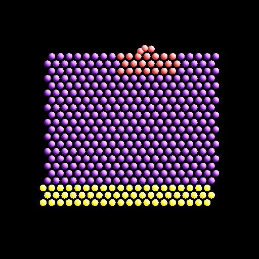
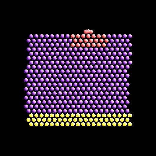
There are 2 Python scripts provided in the tools/python directory, neb_combine.py and neb_final.py, which are useful in analyzing output from a NEB calculation. Assume a NEB simulation with M replicas, and the NEB atoms labeled with a specific atom type.
The neb_combine.py script extracts atom coords for the NEB atoms from all M dump files and creates a single dump file where each snapshot contains the NEB atoms from all the replicas and one copy of non-NEB atoms from the first replica (presumed to be identical in other replicas). This can be visualized/animated to see how the NEB atoms relax as the NEB calculation proceeds.
The neb_final.py script extracts the final snapshot from each of the M dump files to create a single dump file with M snapshots. This can be visualized to watch the system make its transition over the energy barrier.
To illustrate, here are images from the final snapshot produced by the neb_combine.py script run on the dump files produced by the two example input scripts in examples/neb.
Restrictions
This command can only be used if LAMMPS was built with the REPLICA package. See the Build package doc page for more info.
To read compressed files, you must compile LAMMPS with the
-DLAMMPS_GZIP option. See the Build settings doc page for details.
Default
verbosity = default
(HenkelmanA) Henkelman and Jonsson, J Chem Phys, 113, 9978-9985 (2000).
(HenkelmanB) Henkelman, Uberuaga, Jonsson, J Chem Phys, 113, 9901-9904 (2000).
(Nakano) Nakano, Comp Phys Comm, 178, 280-289 (2008).
(Maras) Maras, Trushin, Stukowski, Ala-Nissila, Jonsson, Comp Phys Comm, 205, 13-21 (2016)